Plotting several functions

Question

I'd like to plot a function of one real and one integer variable, but I don't want them all shown in the same 2-D plot - I'd like to see them as separate curves so I can see both "axes", more like how Plot3D works. I'm sure Mathematica can do this, but how?

Edit: Rephrased, I'd like to Plot3D a function of one real and one integer variable. Instead of seeing a surface, I'd like a discrete set of curves in three space.

Answer 1

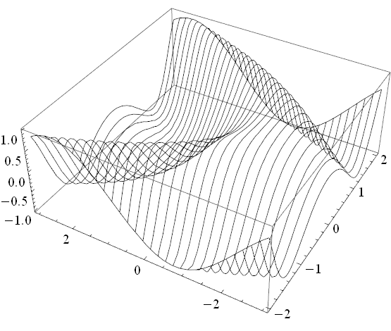
Mesh will do the trick:

Plot3D[Sin[x^2 - y], {x, -2, 2}, {y, -3, 3}, MeshFunctions -> {#2 &}, 
 PlotStyle -> None, Mesh -> 30]

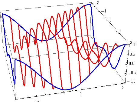
Placing the “wires” on integer values is also easy – see example below. For the range {y, -7, 5} there are 13 integers so you need to ask for 11 wires Mesh -> 11 (in red) because 2 are taken by boundary (blue). With such settings "wires" fall exactly on integer values.

Plot3D[Sin[x^2 - y/2], {x, -2, 2}, {y, -7, 5}, MeshFunctions -> {#2 &}, 
PlotStyle -> None, Mesh -> 11, MeshStyle -> {Thick, Red}, 
BoundaryStyle -> {Thick, Blue}]

Answer 2

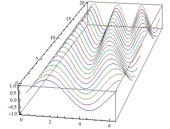
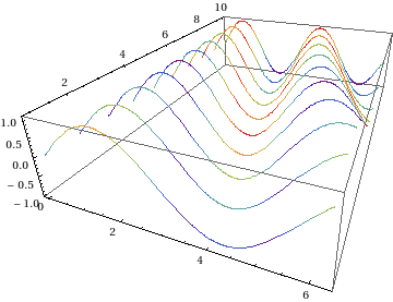
Do you mean something like this?

f[n_, x_] := Sin[x (1 + n/10)]
ParametricPlot3D[Evaluate[Table[{x, n, f[n, x]}, {n, 20}]], {x, 0, 2 Pi}]

Answer 3

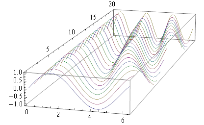
I'm bored, so here is a recreation of Heike's plot without ParametricPlot3D

Graphics3D[
  Table[
    Cases[
      Plot[f[n, x], {x, 0, 2 Pi}],
      Line[x_] :> {ColorData[1][n], Line[{#,n,#2} & @@@ x]},
      {4}
    ],
    {n, 20}
  ],
  Axes -> True
]

Answer 4

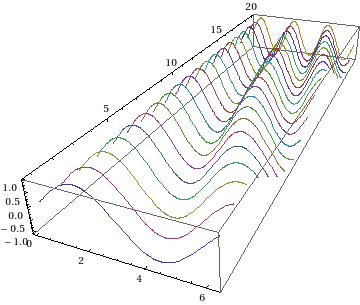
Once upon a time, old versions of Mathematica had a package called Graphics`Graphics3D`, which featured a neat little utility called StackGraphics[] that did exactly what OP wanted. Since the current versions of Mathematica no longer support this package, we are lucky that the upgrading information in the help file features some code for mimicking the functionality of StackGraphics[], which you can easily adapt to your circumstances:

f[n_Integer, x_] := Sin[x (1 + n/10)];
Graphics3D[
 MapIndexed[
  Cases[#, Line[L_] :> {ColorData[1][First[#2]], 
      Line[Thread[{L[[All, 1]], First[#2], L[[All, 2]]}]]}, -1] &, 
  Table[Plot[f[n, x], {x, 0, 2 Pi}], {n, 20}]], Axes -> True, 
 ViewPoint -> {.4, -1., .5}]

---

Of course, if your Plot[]s use the ColorFunction option, stacking graphics is a bit more complicated, since the output internally uses a GraphicsComplex[] object as opposed to a plain Jane Line[]. In that case, something like the following has to be done:

Graphics3D[
 MapIndexed[
  Cases[#1, GraphicsComplex[pts_, rest__] :> 
     GraphicsComplex[Function[pt, Riffle[pt, First[#2]]] /@ pts, rest], -1]&, 
  Table[Plot[f[n, x], {x, 0, 2 Pi}, 
        ColorFunction -> (ColorData["Rainbow"][ArcCos[Cos[Pi (n/5 - #2)]]/Pi]&)],
        {n, 10}]], Axes -> True, ViewPoint -> {.4, -1., .5}]

Answer 5

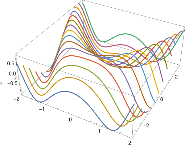
Since v12.3, we have ListLinePlot3D, so we can do something like:

domain = {{-2, 2}, {-3, 3}};

ListLinePlot3D[Array[{x, y} |-> Sin[x^2 - y], {50, 15}, domain]\[Transpose], 
 DataRange -> domain, AxesLabel -> {x, y}]

Alternatively (slower and less elegant, but easier to understand):

{{xL, xR}, {yL, yR}} = {{-2, 2}, {-3, 3}};
pointsx = 50; pointsy = 15;
ListLinePlot3D[
 Table[{x, y, Sin[x^2 - y]}, {y, yL, yR, (yR - yL)/(pointsy - 1)}, {x, xL, xR, (
   xR - xL)/(pointsx - 1)}], AxesLabel -> {x, y}]

Answer 6

Case of explicit functions:

ParametricPlot3D[Evaluate[Table[{ww, zz, Exp[-(ww - 0.5 zz)^2/zz^2]}, 
    {zz, {0.2, 0.4, 0.6, 0.8, 1.0, 1.2}}]], {ww, -2, 2}, 
    PlotStyle -> {{Black, Thick}, {Blue, Thick}, {Red, Thick}, {Yellow, Thick}, 
                  {Green, Thick}, {Magenta, Thick}}]

Case of interpolating functions:

mmax = 4;    
tm = Table[m, {m, 1, mmax}];
tap = {0, 1, 2, 3, 4, 5, 6, 7, 8, 9};
tfp = Table[(n - 1)^m, {m, 1, mmax}, {n, 1, 10}];
tif = Table[{tap[[n]], tfp[[m, n]]}, {m, 1, Length[tfp]}, {n, 1, Length[tap]}]
tg = Table[Interpolation[tif[[m]]], {m, 1, mmax}];
ParametricPlot3D[
    Evaluate[Table[{x, zz, tg[[zz]][x]}, {zz, tm}]], {x, 0, 1}, 
    PlotStyle -> {{Blue, Thick}, {Red, Thick}, {Green, Thick}, {Magenta, Thick}}]