How to plot slices of a surface of an iterative function parametrized by the iterator k? [duplicate]

Question

I am trying to plot a surface of

$$z=\sin^{(k)}(x),\text{where (k) means nesting the function k times}$$

to visualise the fixed points and their neighbourhood to visually analyse their behaviour.

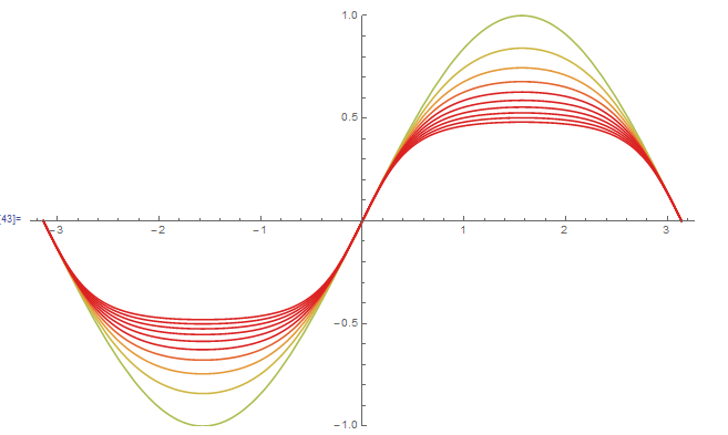
Currently, the following (adapted from this link) give me a contour version of the above:

f[x_] := Sin[x]
Show[Table[Plot[Nest[f, x, i], {x, -π, π}, 
PlotRange -> {-1, 1}, PlotStyle -> ColorData["Rainbow", 0.5 + i/10]], {i, 1, 10}]]

However, I want to space out the contours along the $k$ axis so that e.g. $\sin(x)$ corresponds to $k=1$, $\sin(\sin(x))$ corresponds to $k=2$ and so on...

Below is my most recent attempt at doing it:

 f[x_] := Sin[x]
 data[x_] := Table[{Nest[f, x, i], i}, {i, 0, 10}]
 ListPlot3D[data[x], {x, -π, π}]

which gives me an error

 SetDelayed::write: Tag List in {{x,0},{Sin[x],1},{Sin[Sin[x]],2}, 
{Sin[Sin[Sin[x]]],3},{Sin[Sin[Sin[Sin[x]]]],4},{Sin[Sin[Sin[<<1>>]]],5},
{Sin[Sin[Sin[Sin[Sin[Sin[<<1>>]]]]]],6},
{Sin[Sin[Sin[Sin[Sin[Sin[<<1>>]]]]]],7},
{Sin[Sin[Sin[Sin[Sin[Sin[<<1>>]]]]]],8},
{Sin[Sin[Sin[Sin[Sin[Sin[<<1>>]]]]]],9},
{Sin[Sin[Sin[Sin[Sin[Sin[<<1>>]]]]]],10}}[x_] is Protected. >>

Strangely the data behind seemed to be interpreted correctly

ListPlot3D[{{x, 0}, {Sin[x], 1}, {Sin[Sin[x]], 2}, {Sin[Sin[Sin[x]]], 
3}, {Sin[Sin[Sin[Sin[x]]]], 4}, {Sin[Sin[Sin[Sin[Sin[x]]]]], 
5}, {Sin[Sin[Sin[Sin[Sin[Sin[x]]]]]], 
6}, {Sin[Sin[Sin[Sin[Sin[Sin[Sin[x]]]]]]], 
7}, {Sin[Sin[Sin[Sin[Sin[Sin[Sin[Sin[x]]]]]]]], 
8}, {Sin[Sin[Sin[Sin[Sin[Sin[Sin[Sin[Sin[x]]]]]]]]], 
9}, {Sin[Sin[Sin[Sin[Sin[Sin[Sin[Sin[Sin[Sin[x]]]]]]]]]], 10}}[x], {x, -\[Pi], \[Pi]}]

I was suspecting that ListPlot3D cannot read my input is probably because I have mixed data type. In details

$$z\in \mathbb{R}$$ $$x \in [-\pi,\pi]$$ but $$k \in \{0,1,2,3,4,5,6,7,8,9,10\}$$

From browsing the documentation, I am not aware of any examples of plots made from a mix of discrete and continuous variables as plotting arguments, thus I am not sure how to plot the surface I want.

I am not sure how to circumvent/cheat it without taking too much computation time since if my set of points $x$ is too sparse, it will fail to display the sinusoidal feature (which will be a problem because I am planning to apply this code on other iterative functions, such as the logistic map), but if my sampling is too dense, it will probably took too much computation time

Any ideas on what I can do?

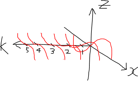
P.S. To give an idea on what I am trying to achieve, refer to the below sketch:

which after interpolation along $k$, will give a nice surface.

Answer 1

Use Interpolation if you want a regular function. Just for the plot you can also use ListPlot3D.

fun = Interpolation[
Flatten[Table[{x, k, Nest[Sin, x, k]}, {x, -Pi, Pi, .1}, {k, 1, 10,1}], 1]];

Plot the continuous function and those $k$-mesh lines!

Plot3D[fun[x, k], {x, -Pi, Pi}, {k, 1, 10}, MeshFunctions -> {#2 &}, 
 Mesh -> 10, PerformanceGoal -> "Quality", MeshStyle -> {{Black, Thin}}]

Answer 2

If you only want discrete lines you can use ParametricPlot3D in combination with Map or Table embedded in a Show.

Below the Blend function is used to add a variable color (optional). Black is Sin[x] and Red is the curve nested ten times.

Show[
 Map[
  ParametricPlot3D[{u, #, Nest[Sin, u, #]}, {u, -\[Pi], \[Pi]},
    PlotStyle -> Blend[{Black, Red}, #/10],
    PlotRange -> {{-\[Pi], \[Pi]}, {0, 10}, {-1, 1}}
    ] &,
  Range[10]
  ]
 ]

Answer 3

This is, I think, a dupe of Plotting several functions, except that that thread displayed only the contours.

An approach simpler than the other posted answers proceeds like so:

Plot3D[Nest[Sin, x, Round[k]], {x, -π, π}, {k, 1, 10},
       MeshFunctions -> {#2 &}, Mesh -> 10]