11
$\begingroup$

I plotted recently some figures in Matlab and their quality was not that satisfactory, so I come to Mathematica as my supervisor suggested. This is how such figure looks like in Matlab:
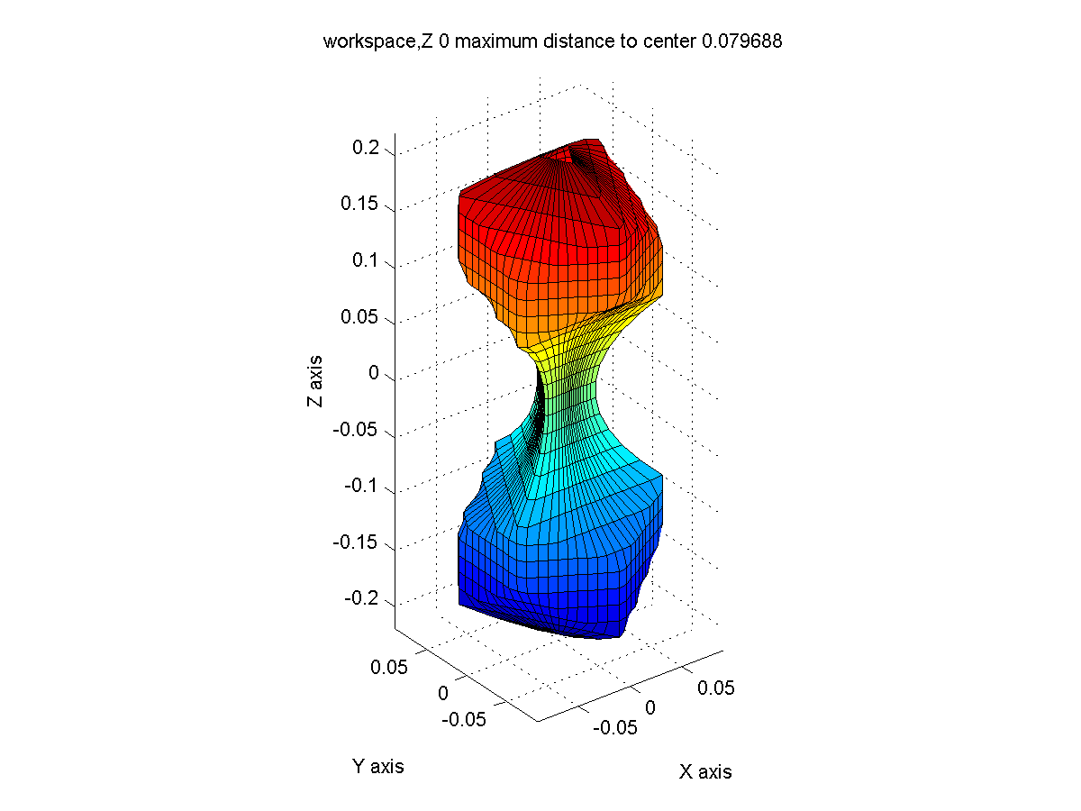
The data plot from matlab.

In Matlab, I have three m by n matrices A,B,C, whose entries in the corresponding position are the calculated x,y,z coordinates of the points on the surface correspondingly. And each row of the 3 matrices corresponds to different Z value, so the C matrix's each row has identical entries. Then I used surf function to plot.

But when I have the same plot in Mathematica, it gives me something like this:
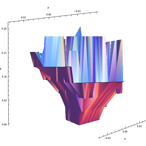
The upper half of the same surface.

First I used Flatten function to put my 3 matrices into a triple form, then plotted only the upper half of the figure, and realized the upper part of the surface won't close as I expected, I guess this is because for each XY pair, it may have more than one corresponding Z values (since it looks like a sphere), and the sample data points that with closest xy values are connected first. So some of the data points on the top are connected to the lower parts data points whose xy are closer to them, rather than connected to where it should.

Right now I'm using ListPlot3D command. BTW, I got those data by using a outer loop to search the Z values and for each Z value, I used polar coordinates to characterize the contour, then transform it into Cartesian form, so I can't get uniform XY.

I'm wondering if there is any options or way to deal with this situation, or any way to Plot 3 matrices like the surf function in Matlab?


Follow Up 1

Thanks a lot for everyone's answer, I'd like to upload the code, but the code is actually very lengthy, and not possible to copy it in this poster, is there any method to upload the file?

Or to make the long story short, I have a 300 by 3 matrix, i.e. 300 triples as the input of ListPlot3D (or other possible function like the SurfacePlot3D), and the triples hold the values like {{1.234,0,0},{1.200,0.0003,0},{1.150,0.007,0},...,{1.224,-0.003,0},{1.4,0,0.3},{1.340,0.0003,0.3},{1.250,0.007,0.3}...,{1.358,-0.003,0.3},...}, the last value represent Z coordinates Z=z_i, and the first two are obtained by first obtaining the polar coordinates of the data points on the contour Z=z_i, and then transforming them into cartesian coordinates.


Follow Up 2

Thanks a lot for your answers, I realize I could share it with dropbox, here is the link: https://www.dropbox.com/sh/2h722qxalkecupk/AADA6IUiPZA2MD-0cSXx0eiAa?dl=0;

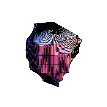
I've tried the commands you guys mentioned in the above file: For the paramterplot3d function from Rahul Narain, it works perfect for my problem, and gave me this figure:
enter image description here

This is exactly how it should be, but looks a bit poor, any idea of improving the quality by eliminating the mesh on the figure and make it smoother if possible?

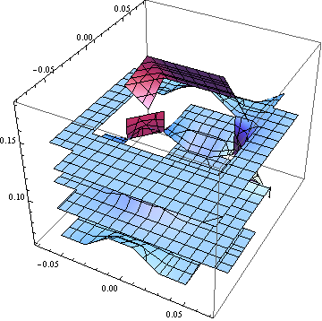
I also tried the ListSurfacePlot3D function, seems it's also exactly for this application, and quite powerful, but it gives me some result like this:
enter image description here

Any ideas?

And the answer to you mean you are just plotting the surface f(x,y)=c? from Igor Rivin is: not exactly, for I have triples and Z values changes.


Follow Up 3

Hello guys, I've tried your codes, all of them work great!

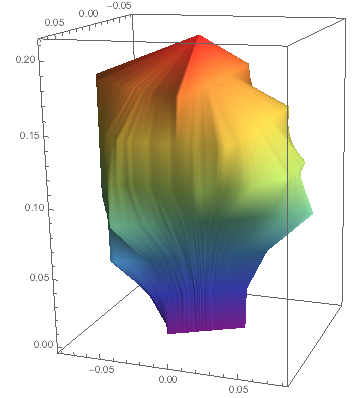
Problem is more or less solved, but if possible, I'd also like to ask again if anyone can help with the third figure in this thread, to eliminate the grids on the surface? And even better if we can make the surface a little bit smoother? This surface represents the data a bit more precise than the one gained by interpolation, which is obtained by the listParametricPlot3D function. I also have it in my uploaded file. But anyway, the interpolation method also works great, but it's a bit ,thanks a lot! Hello, everyone, problem solved, all of your answers work great, just I can just pick one answer.

$\endgroup$
10
  • 2
    $\begingroup$ It may be that few site users will know what the surf function does. I'm afraid I find the description of the problem hard to follow. Maybe someone will know what you want. Would it be convenient for you to post the code you tried? $\endgroup$
    – Michael E2
    Commented Sep 21, 2014 at 2:24
  • 2
    $\begingroup$ That Mathematica plot is quite literally the ugliest thing I have ever seen in all my years of programming on Mathematica. In fact, it's so mind-bendingly grotesque that I actually would love to see the source code, just to have the opportunity to horrify my friends. +1 $\endgroup$ Commented Sep 21, 2014 at 2:30
  • $\begingroup$ ListSurfacePlot3D might be better for this case.. $\endgroup$
    – halmir
    Commented Sep 21, 2014 at 2:52
  • 1
    $\begingroup$ Without the MATLAB code and the data, this seems impossible to answer. $\endgroup$
    – Igor Rivin
    Commented Sep 21, 2014 at 2:59
  • $\begingroup$ Thanks a lot for your answers, and I'm wondering how I can upload the code file? Since the code is very lengthy to be put in the thread, thanks a lot! $\endgroup$
    – larry
    Commented Sep 21, 2014 at 3:18

3 Answers 3

10
$\begingroup$

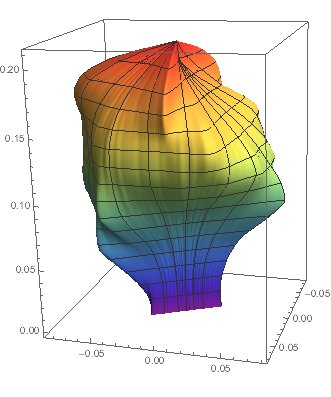
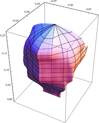
(Updated to show no mesh.) The data seems to have been converted from polar coordinates. One can convert it back and interpolate, with an appropriate interpolation order. Below I show orders 1 and 3 (3 is the default).

polardata = {{#4, #3}, Norm[{#1, #2}]} & @@@ 
   Transpose[{
     Flatten[xx], Flatten[yy], Flatten[zz], 
     Flatten@
      ConstantArray[
       ReplacePart[Apply[ArcTan, Transpose[{xx, yy}, {3, 1, 2}][[1]], {1}], 1 -> N[-Pi]],
       Length[Transpose[{xx, yy}, {3, 1, 2}]]]
    }];

r1 = Interpolation[polardata, InterpolationOrder -> 1];
r = Interpolation[polardata];

ParametricPlot3D[
 r1[t, z] {Cos[t], Sin[t], 0} + {0, 0, z}, {z, 0, 0.21}, {t, -Pi, Pi},
  PlotPoints -> Dimensions[xx], MaxRecursion -> 0, Mesh -> None,
  ColorFunction -> "Rainbow"]

Mathematica graphics

ParametricPlot3D[
 r[t, z] {Cos[t], Sin[t], 0} + {0, 0, z}, {z, 0, 0.21}, {t, -Pi, Pi}, 
 PlotPoints -> Dimensions[xx], ColorFunction -> "Rainbow"]

Mathematica graphics

To eliminate the mesh lines, use the option Mesh -> None.

To give a polygonal rendering (to remove the automatic surface smoothing done by the front end), use the option NormalsFunction -> None.

I think the ragged surface is due to the data itself. Otherwise it's not so clear what the OP finds unsatisfactory about the Matlab plot.

$\endgroup$
7
$\begingroup$

A simpler approach:

{m, n} = Dimensions[xx];
fx = Interpolation[Flatten[Table[{{i, j}, xx[[i, j]]}, {i, m}, {j, n}], 1]];
fy = Interpolation[Flatten[Table[{{i, j}, yy[[i, j]]}, {i, m}, {j, n}], 1]];
fz = Interpolation[Flatten[Table[{{i, j}, zz[[i, j]]}, {i, m}, {j, n}], 1]];
ParametricPlot3D[{fx[i, j], fy[i, j], fz[i, j]}, {i, 1, m}, {j, 1, n}, PlotPoints -> 50]

enter image description here

I do agree with @Michael E2 that the ragged surface is an artifact of the data itself. If you compare the mesh in the Matlab plot to the mesh in the second Mathematica plot in the question, you can see that the latter has far more samples in the horizontal direction. I'm not sure we're working with the same data that was used to create the Matlab plot.

$\endgroup$
5
$\begingroup$

The OP's listParametricPlot3D constructs nonplanar quadrilaterals (Polygons) for a GraphicsComplex with

Polygon[Flatten[
  Table[{1 + i + xx j, 2 + i + xx j, 2 + i + xx (j + 1), 1 + i + xx (j + 1)},
   {j, 0, yy - 2}, {i, 0, xx - 2}], 1]]

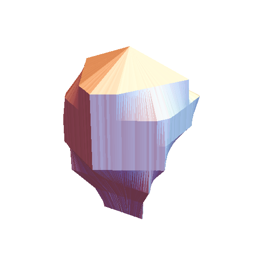
where xx, yy are the dimensions of the tensor grid for the surface in the OP's data. One problem with nonplanar polygons is that the Front End has trouble deciding which face of the polygon is facing the viewer. This easily observed by rotating the figure while focusing on the edges of the image. It is better to use triangles, for which there is no ambiguity. The use of EdgeForm to remove the surface grid has been mentioned by Rahul Narain in a comment.

dataMatrix = Transpose[{xx, yy, zz}, {3, 1, 2}];
Dimensions[dataMatrix];
listParametricPlot3D[points_, opt___?OptionQ] := 
 Module[{xx, yy}, {yy, xx} = Take[Dimensions[points], 2];
  Graphics3D[
   GraphicsComplex[
    Join @@ points,
    {EdgeForm[], Polygon[Flatten[
       Table[{
           {1 + i + xx j, 2 + i + xx j, 2 + i + xx (j + 1)},
           {1 + i + xx j, 2 + i + xx (j + 1), 1 + i + xx (j + 1)}},
         {j, 0, yy - 2}, {i, 0, xx - 2}], 
       2]]}], opt]]

gr = listParametricPlot3D[dataMatrix, Boxed -> False, 
  SphericalRegion -> True]

Mathematica graphics

The triangles are evident because there are no VertexNormals. Another issue already remarked on by Rahul and me is some apparent noise in the data that makes the surface look slightly ragged or striated. This exaggerates the appearance of shadows.

The OP expressed a wish for a smoother surface. The plot of the linear interpolation, r1 with InterpolationOrder -> 1, in my other answer produces exactly the same shape as in this answer, except with vertex normals (and coloring, mesh, and perhaps other trivial differences). The vertex normals cause the surface to be rendered as somewhat smoother, but obviously not completely smooth. The higher-order interpolation r also tends to smooth out the surface, but this, too, seemed unsatisfactory for some reason. One thing that is unclear is whether some corners are meant to be corners and not be smoothed. If so, it would seem that automatic smoothing of the surface will be difficult to achieve. The smoothing may have to be achieved by modifying the data to align points that appear to be nearly collinear in the image. I do not know of an automatic way to achieve that either.


Edit

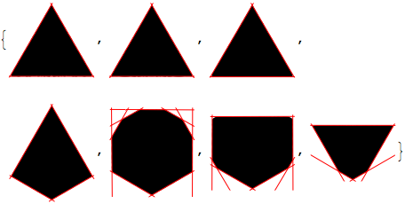
If we assume that the approximately straight edges are actually straight, we can apply some image processing and ImageLines to smooth some of the surface. It will reveal that next-to-bottom levels of the data are perhaps not aligned with the bottom.

The 6th level was particularly difficult and needed special treatment to get the oblique lines near the bottom of the sides (below). Otherwise ImageLines did a pretty good job. I used Alexey Popkov's completePlotRange to rescale the image coordinates to the data coordinates.

completePlotRange[plot : (_Graphics | _Graphics3D | _Graph)] := 
  Last@Last@
    Reap[Rasterize[
      Show[plot, Axes -> True, Frame -> False, 
       Ticks -> ((Sow[{##}]; Automatic) &), 
       DisplayFunction -> Identity, ImageSize -> 0], 
      ImageResolution -> 1]];

dataMatrix = Transpose[{xx, yy, zz}, {3, 1, 2}];

gr = Graphics[Polygon[#]] & /@ dataMatrix[[1 ;; 7, All, 1 ;; 2]];
im = Image /@ gr;
im[[6]] = Image[gr[[6]], ImageSize -> 1000];

lines = Transpose[#, {3, 2, 1}] & /@ 
   MapThread[
    Rescale, {Transpose[
        ImageLines[Thinning@Binarize@GradientFilter[#, 2] &@#, 
         If[First@ImageDimensions[#] >= 800, 0.04, 0.08]], {3, 2, 
         1}] & /@ im, Thread[{0, ImageDimensions[#]}] & /@ im, 
     completePlotRange /@ gr}, 2];
MapThread[
 Show[#1, Graphics[{Red, PointSize[Large], Line[#2]}],
   PlotRange -> All
   ] &, {gr, lines}]

Mathematica graphics

We use the lines found above with RegionNearest to project the data points onto the nearest line. Points further away from the nearest line than threshold are not changed.

threshold = 0.0015;
smoothData = MapThread[
    Function[{datalevel, line},
     Map[With[{p = RegionNearest[Line@line, Most@#]~Append~Last[#]}, 
        If[EuclideanDistance[p, #] <= threshold, p, #]] &, datalevel]
     ],
    {dataMatrix[[1 ;; 7]], lines}]~Append~Last[dataMatrix];

listParametricPlot3D[smoothData, Boxed -> False, 
 SphericalRegion -> True]

Mathematica graphics

I'm not sure if that is what the OP had in mind, but it smooths some of the surfaces.

$\endgroup$

Your Answer

By clicking “Post Your Answer”, you agree to our terms of service and acknowledge you have read our privacy policy.

Not the answer you're looking for? Browse other questions tagged or ask your own question.