56
$\begingroup$

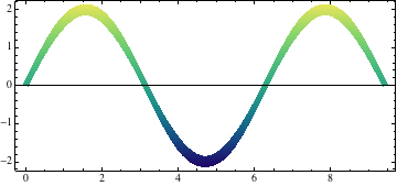
I know, that I can change the color of a function with the help of PlotStyle:

Plot[Sin[x], {x, 0, 3 Pi}, PlotStyle -> {Green, Thickness[0.01]}]

I also know, that I can vary the color in relation to the function value:

Plot[Sin[x], {x, 0, 3 Pi}, PlotStyle -> {Thickness[0.01]}, 
 ColorFunction -> "BlueGreenYellow"]

I wonder if it is possible to change the thickness of a plotted function dependent on the function value, for example the absolute value of the function.

For the example above a nice thing would be to have, that the line is e.g. twice as thick at the minima and the maxima as it is at the roots.

$\endgroup$
4

5 Answers 5

30
$\begingroup$

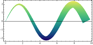
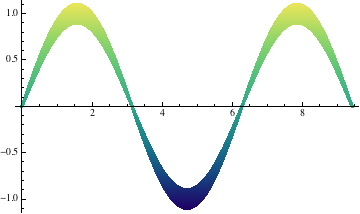
Another way is to use ParametricPlot (which will accomplish an equivalent thing via polygons). Here, thickness adds a multiple th of the unit normal to the curve. Just pass a thickness function as the parameter th.

thickness[f_, th_] := Block[{x}, {x, f} + Normalize[{-D[f, x], 1}] th];
ParametricPlot[
 Evaluate@thickness[2 Sin[x], 0.075 (1 + Sin[x]^2) t],
 {x, 0, 3 Pi}, {t, -1, 1},
 Mesh -> None, BoundaryStyle -> None, 
 ColorFunction -> (ColorData["BlueGreenYellow"][#2] &)]

Mathematica graphics


Update

This is a nicer interface. You pass the thickness function as an option. The function will have one parameter passed to it, namely the variable var of the plot.

ClearAll[thicknessPlot];
SetAttributes[thicknessPlot, HoldAll];
Options[thicknessPlot] = {thicknessFunction -> (0.1 &)} ~Join~ Options[ParametricPlot];
thicknessPlot[f_, {var_, v1_, v2_}, opts : OptionsPattern[]] := 
 Module[{param},
  With[{thicknessFn = OptionValue[thicknessFunction], 
        unitN = Block[{var}, Normalize[{-D[f, var], 1}]]},
   ParametricPlot[{var, f} + thicknessFn[var] unitN param,
    {var, v1, v2}, {param, -1, 1},
    Mesh -> (OptionValue[Mesh] /. Automatic -> None), 
    BoundaryStyle -> (OptionValue[BoundaryStyle] /. Automatic -> None),
    Evaluate @ FilterRules[FilterRules[{opts}, Options[ParametricPlot]], 
      Except[Mesh | BoundaryStyle]]
    ]]
  ]

Example:

thicknessPlot[2 Sin[x], {x, 0, 3 Pi}, 
 thicknessFunction -> (0.01 + #/20 &), 
 ColorFunction -> (ColorData["BlueGreenYellow"][#2] &)]

Mathematica graphics

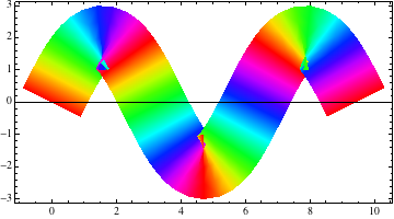
Note: Adding PlotPoints -> {15, 2} will speed things up, or if more points are needed for a complicated graph, then something like PlotPoints -> {50, 2}. Since the formula in ParametricPlot is a linear function of the thickness parameter param, two plot points for that dimension will usually be enough.

Also note that if half the thickness exceeds the radius of curvature, the curve will fold over itself. This is a problem with the mathematics, not the code (except that the code implements the mathematics).

thicknessPlot[2 Sin[x], {x, 0, 3 Pi}, thicknessFunction -> (1 &), 
 PlotPoints -> {15, 2}, ColorFunction -> (Hue[4 #3] &)]

Mathematica graphics

$\endgroup$
4
  • $\begingroup$ Basically we had the same idea, only that it took me an hour to write my one up :-) $\endgroup$
    – halirutan
    Commented Jul 7, 2013 at 2:26
  • $\begingroup$ @halirutan I rushed mine because of home life -- and didn't see yours or your comment until I was done with my update. I've used this idea before, but I guess it hasn't come up on this site yet. $\endgroup$
    – Michael E2
    Commented Jul 7, 2013 at 4:35
  • $\begingroup$ This is a good idea. Your last updated example is not working here when I copy the code. $\endgroup$
    – abrhv
    Commented Jul 7, 2013 at 11:46
  • $\begingroup$ @abrhv Sorry about that. I had modified the definition, but forgot to update the code for the example. Thanks. $\endgroup$
    – Michael E2
    Commented Jul 7, 2013 at 12:39
38
$\begingroup$

I see at least two problematic points here. The first and most obvious is, that Plot creates many Line directives. If you set the thickness of adjacent lines differently, you may get thickness-jumps where the lines meet. In the worst case something like this

Graphics[{Thickness[0.01], Line[{{0, 0}, {1, 1}}], Thickness[0.05], 
  Line[{{1, 1}, {2, 0}}]}]

Mathematica graphics

Another point is, that adjacent lines are not really connected smoothly. Let me give a very verbose, but complete manual approach which can, once understood, later be used to transform an existing plot as in Cuba's answer.

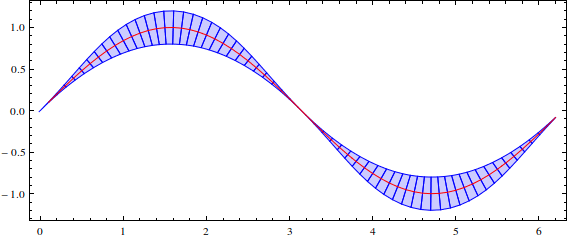
What we will do is to draw a series of polygons which connect smoothly and let us specify the thickness exactly in dimensions of the coordinate system. Here an example of what we try to achieve

Mathematica graphics

I will use your Sin[x] example, but the approach can be generalized to different functions. As you see above the polygons need lines which are perpendicular to your function. Let us start by transforming your function $y=sin(x)$ into parametric form. This will help later if you try this with more evil functions. All points on the graph are given by the parametric function

$$f(t)=\left(\begin{array}{c}t\\sin(t)\end{array}\right)$$

To create exact thicknesses we need the normalized vector which is perpendicular to your graph. This is simply the gradient rotated about 90 degree and then normalized (many people won't need Mathematica for this, but lets do it anyway):

f[t_] := {t, Sin[t]}
df[t_] = Normalize[RotationMatrix[Pi/2].D[f[t], t]]

Now we can create the from two adjacent times t1 and t2 a polygon with 4 vertices. In the above graphics, you see the sine function as red in the middle and if you leave this out, you see the graphics contains only polygons with 4 vertices.

If you look at one such polygon, we will draw it counter-clockwise starting with the lower-left corner. This means taking the point at t1 and going half the thickness along the negative perpendicular gradient. The next point is the same for t2 and the other points are equivalent with the difference that we move along the positive perp. gradient. This can verbosely be written as

points[{t1_, t2_}, tfunc_] :=
 {f[t1] - tfunc[t1]*df[t1]/2,
  f[t2] - tfunc[t2]*df[t2]/2,
  f[t2] + tfunc[t2]*df[t2]/2,
  f[t1] + tfunc[t1]*df[t1]/2
 }

The function tfunc is here our thickness-function which will be evaluated at each time to give us the wanted thickness.

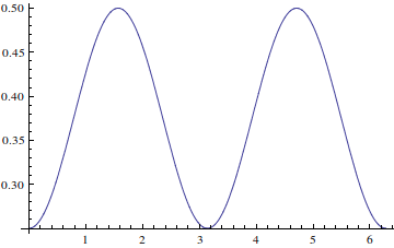
Now we are ready to test. Lets say we want our sine to be 0.25 at the roots and 0.5 at the extreme points, then a thickness function could look like:

thickF[t_] := .25 Sin[t]^2 + 0.25;
Plot[thickF[t], {t, 0, 2 Pi}]

Mathematica graphics

For this simple test we use fixed sampling points but nevertheless the curve looks quite smooth

times = Table[t, {t, 0, 2 Pi, 0.1}];
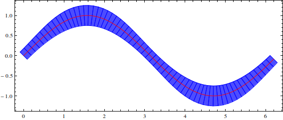
Graphics[{Blue, FaceForm[Opacity[0.7]], EdgeForm[Blue], 
  Polygon /@ (points[#, thickF] & /@ Partition[times, 2, 1]), Red, 
  Line[f /@ times]}, Axes -> False, Frame -> True]

Please note that the work is done in points[#, thickF] & /@ Partition[times, 2, 1], the rest is show.

Mathematica graphics

Since the approach uses parametric representation, you can now easily handle curves which are not one-to-one functions.

f[t_] := {Sin[t] + 2 Sin[2 t], Cos[t] - 2 Cos[2 t]};
df[t_] = Normalize[RotationMatrix[Pi/2].D[f[t], t]];
thickF[t_] := 0.2 (-Sin[3 t] + 1) + 0.1;

times = Append[#, First[#]] &@Table[t, {t, 0, 2 Pi, 0.01}];
Graphics[{Blue, FaceForm[Opacity[0.7]], 
  Polygon /@ (points[#, thickF] & /@ Partition[times, 2, 1])}]

Mathematica graphics

$\endgroup$
6
  • $\begingroup$ Related: mathematica.stackexchange.com/a/13376/5 $\endgroup$
    – rm -rf
    Commented Jul 7, 2013 at 4:51
  • $\begingroup$ @rm-rf If this is related then mine is a duplicate of that. But believe me, I haven't seen this Q&A before :) $\endgroup$
    – Kuba
    Commented Jul 7, 2013 at 7:23
  • $\begingroup$ A nice explanation. (+1) You might add Method -> {"TransparentPolygonMesh" -> True} to get rid of the Moiré effect. A slight criticism: The corners of the quadrilaterals are calculated twice, except at the ends. $\endgroup$
    – Michael E2
    Commented Jul 7, 2013 at 12:56
  • $\begingroup$ @MichaelE2 I was aware of the double calculation but left it in order to keep the explanations simple. Where do I have to put the Method option? Because on my Linux box I don't see any difference when I append it as option to Graphics. $\endgroup$
    – halirutan
    Commented Jul 7, 2013 at 13:06
  • $\begingroup$ Yes, put the Method with the Graphics. (See this.) I figured that about the double calculation, and it does help the explanation be very clear. Still, the next person might want to make it more efficient. $\endgroup$
    – Michael E2
    Commented Jul 7, 2013 at 13:17
32
$\begingroup$

the newest edit

thicknessFunction is not compatibile with ColorFunction. It is because Mathematica is creating GraphicsComplex for plots with ColotFunction.

I have created procedure which is dealing with it. It is more useful than thicknessFunction[f_, f2_] from the bottom of this post because MMA is taking care for scalling etc.

thick$color[f_] := ReplaceAll[#, 
            GraphicsComplex[x_List, y_List, z : OptionsPattern[__]] :> 
            GraphicsComplex[
              x, 
              (y /.Line[x2_List,z2 : OptionsPattern[]] :> (Sequence @@ (
                       {Thickness[f @@ (Mean /@Transpose[x[[#]]])], 
                       Line[#, VertexColors -> Automatic]} & /@ Partition[x2, 2, 1]))),
              z]] &;

ParametricPlot[{Sin[t]+2 Sin[2 t], Cos[t]-2Cos[2t]}, {t, 0,3 Pi}, PlotPoints -> 500, 
               MaxRecursion -> 1, Axes -> False, ColorFunction -> "Rainbow"
              ] //  thick$color[.01 (Abs[#1 #2]) &]

enter image description here

ParametricPlot[{Sin[t]+Sin[15t], Cos[t]-Cos[15t]}, {t, 0, 3 Pi},PlotPoints -> 2000,
               MaxRecursion -> 1, Axes -> False, ColorFunction -> "DarkRainbow"
              ] //  thick$color[.01 (Norm[{##}]) &]

enter image description here


Before last edit

With Your request:

[...] twice as thick at the minima and the maxima as it is at the roots. [...]

Artes's approach seems to be natural, because You can implement thickness dependance of function absolute value, function's derivative, or even argument value just by including those into first list in Plot.


However, it could be challenging if one does not feel good in analysis.

I think it is a good moment to try to create something like ColorFunction for plot thickness. It is my solution:

thicknessFunction[f_] :=  ReplaceAll[#, Line[x__] :> (
   {AbsoluteThickness[f @@ (Mean /@ Transpose[#])], Line@#} & /@ Partition[x, 2, 1])] &

OP's function case

In Your case such function should have form f = Function[{x,y}, 7 + 7 Abs[x]]. Then thickness for y = 0 is 7 and twice as much, 14, for y = 1. So simple because Sin is quite predictable :).

Following example is for 3 times thicker at extremes (just for clarity).

f = Function[{x, y}, 5 + 10 Abs[y]]
Plot[Sin[x], {x, 0, 3 Pi}, PlotPoints->500, MaxRecursion->1] // thicknessFunction[f]
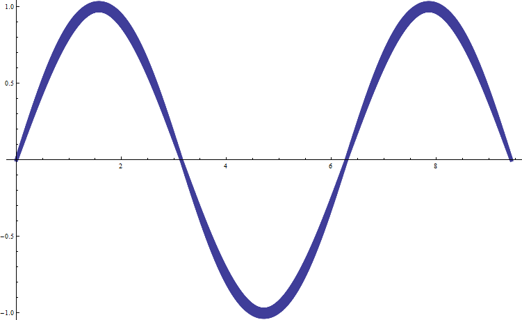
enter image description here

Explanation

Note that many PlotPoints and MaxRecursion->1 is a must for smooth result. thicknessFunction is working on sample points and if we want smooth plot we need many but quite uniformly sampled points. Take a look:

(Plot[5 Sin[x], {x, 0, 10 Pi}, ImageSize -> 300, PlotPoints -> #1, 
 MaxRecursion -> #2] /. Line -> Point) & @@@ {{100, Automatic}, {100, 1}, {500, 1}}

enter image description here Then we have to just replace those points to lines with thickness specified by us.

Examples

y = x with thickness proportional to x^2 and x

plot = Plot[x, {x, 0, 30}, AspectRatio -> 1, PlotPoints -> 500, MaxRecursion -> 1,   
            ImageSize -> 300];
plot // thicknessFunction[.4 #1^2 &]
plot // thicknessFunction[2 #1 &]

OP's case variations. Even including some analysis.

plot = Plot[Sin[2 x], {x, 0, 3 Pi}, PlotPoints -> 500, MaxRecursion -> 1, 
            PlotRange -> {{-2, 12}, {-1.5, 1.5}}, Frame -> True, Axes -> False];
plot // thicknessFunction[Abs[10 Sin'[2 #1]] + 2 #1 &]
plot // thicknessFunction[10 (#2 + 1) &]

Limitations

I have not tested it with all graphics functions in Mathmematica :) so I have to assume it is not bulletproof.

Important remark - it will not cooperate with ColorFunction but:

color plot

Stealing halirutan's example lets implement colors:

thicknessFunction[f_, f2_] := ReplaceAll[#, Line[x__] :> (
                                    {Blend["Rainbow", f2 @@ (Mean /@ Transpose[#])], 
                                     Thickness[f @@ (Mean /@ Transpose[#])],
                                     Line@#} & /@ Partition[x, 2, 1])] &

ParametricPlot[{Sin[t] + 2 Sin[2 t], Cos[t] - 2 Cos[2 t]}, {t, 0, 3 Pi},
               PlotPoints -> 2000, MaxRecursion -> 4, Axes -> False, ImageSize -> 500
              ] //  thicknessFunction[.01 (Abs[#1 #2]) &, Abs[#2/2] &]

This have to be optimized and I must work on scalling etc. But do not have time now :(

$\endgroup$
3
  • $\begingroup$ May I use a modified version of the above thick$color in a coding project licensed under MIT-0 (much more permissive than CC BY-SA 3.0 for this post)? I will of course link this answer in the comments. $\endgroup$
    – yawnoc
    Commented Mar 15, 2021 at 10:23
  • 1
    $\begingroup$ @yawnoc sure, I got lost in recent SE licensing updates but as long SE does not mind, I don't either. $\endgroup$
    – Kuba
    Commented Mar 15, 2021 at 10:56
  • $\begingroup$ Thank you! As far as I am aware, you are free to re-license your own content under any alternative license you want (whether more or less permissive); it's just that you can't revoke the CC permissions granted to SE. $\endgroup$
    – yawnoc
    Commented Mar 15, 2021 at 11:09
19
$\begingroup$

If you want to combine the thickness with the color information, you could do this:

Plot[{1.1 Sin[x], .9 Sin[x]}, {x, 0, 3 Pi}, 
 PlotStyle -> {Thickness[0.01]}, ColorFunction -> "BlueGreenYellow", 
 Filling -> {1 -> {2}}]

thickness

Thanks Kuba for pointing out Artes' answer that shows how Filling can work here.

Edit

In response to the comment, let me suggest something completely different: do the whole thing in three dimensions, and use the fact that one can draw 3D lines as Tube which allows the specification of a varying radius at each intermediate point along the line. Here, the calculation of the perpendicular directions to the curve is already done for us:

makeTube[p_, width_: .1, color_: Darker[Blue]] := 
 Graphics3D[{color, 
     Tube[#, width Abs[#[[All, 2]]]] &@
      First[Map[Append[#, 0] &, 
        First@Cases[Normal[#], _Line, Infinity], {2}]]}, 
    Boxed -> False, Axes -> {True, True, False}, 
    AxesOrigin -> {0, 0, 0}, ViewPoint -> {0, 0, 10000}, 
    ViewVertical -> {0, 1, 0}, Lighting -> "Neutral"] &[p]

makeTube[Plot[Sin[x], {x, 0, 3 Pi}]]

3d plot

As a Graphics3D object, this by default has AspectRatio -> Automatic, which is needed to avoid distortion of the thickness.

Here, I've chosen the ViewPoint and ViewVertical to make the result look like a 2D plot. This may be cheating, but maybe you can use the idea if at some point you want to include a third dimension...

The function makeTube assumes that the argument p contains a Line as it would be generated by the standard Plot command. One could add more logic to analyze p, in case it contains more than one Line, etc. But this is just a proof of principle.

$\endgroup$
4
  • $\begingroup$ Thanks for the answer. I had hoped for a way to specify the exact thickness of the line. To make more clear what I mean, I have edited my answer and specified the example further. $\endgroup$
    – abrhv
    Commented Jul 6, 2013 at 23:24
  • $\begingroup$ Thanks for the idea with the tube. I think in real cases I wouldn't use it, but it is a nice alternative. $\endgroup$
    – abrhv
    Commented Jul 7, 2013 at 11:40
  • $\begingroup$ The Tube idea is a good one. It also takes VertexColors, so it can potentially have varying colors. For the view point, one could also use ViewPoint -> Top. $\endgroup$
    – Michael E2
    Commented Jul 7, 2013 at 13:25
  • $\begingroup$ @MichaelE2 Thanks for pointing out Top, it must have slipped my mind. $\endgroup$
    – Jens
    Commented Jul 7, 2013 at 17:36
15
$\begingroup$

Another, fairly general way to approach this is to discretize the plot into points, which can then be controlled at will. For example, with the OPs Sine function:

data = Table[{x, Sin[x]}, {x, 0, 3 Pi, 0.01}]; 
Graphics[Point[data]]

enter image description here

To vary the size of the individual points:

allPointsSize = Table[{PointSize[data[[i, 1]]/300], 
                       Point[data[[i]]]}, {i, 1, Length[data]}];
Graphics[allPointsSize]

enter image description here

To vary both the size and color:

allPointsColor = Table[{PointSize[data[[i, 1]]/300], 
                 Hue[i/Length[data]],  Point[data[[i]]]}, {i, 1, Length[data]}];
Graphics[allPointsColor]

enter image description here

Applying this to Halirutan's parametric swirl function:

swirl = Table[{Sin[t] + 2 Sin[2 t], Cos[t] - 2 Cos[2 t]}, {t, 0, 3 Pi, 0.01}];
allPointsSwirl = Table[{PointSize[100 Abs[swirl[[i, 1]]]/Length[swirl]], 
       Hue[i/Length[swirl]], Point[swirl[[i]]]}, {i, 1, Length[swirl]}];
Graphics[allPointsSwirl]

enter image description here

$\endgroup$
1
  • $\begingroup$ One interesting property of this approach is that the colouring is also "rounded". Compare i.sstatic.net/4zmXK.png and i.sstatic.net/s4O0j.png, where the only difference is reversing the order of points. Note the shape of the green/orange transition. $\endgroup$
    – user484
    Commented Apr 1, 2014 at 16:58

Your Answer

By clicking “Post Your Answer”, you agree to our terms of service and acknowledge you have read our privacy policy.

Not the answer you're looking for? Browse other questions tagged or ask your own question.