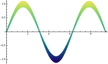
If you want to combine the thickness with the color information, you could do this:
Plot[{1.1 Sin[x], .9 Sin[x]}, {x, 0, 3 Pi},
 PlotStyle -> {Thickness[0.01]}, ColorFunction -> "BlueGreenYellow",
 Filling -> {1 -> {2}}]

Thanks Kuba for pointing out Artes' answerArtes' answer that shows how Filling can work here.
Edit
In response to the comment, let me suggest something completely different: do the whole thing in three dimensions, and use the fact that one can draw 3D lines as Tube which allows the specification of a varying radius at each intermediate point along the line. Here, the calculation of the perpendicular directions to the curve is already done for us:
makeTube[p_, width_: .1, color_: Darker[Blue]] :=
 Graphics3D[{color,
     Tube[#, width Abs[#[[All, 2]]]] &@
      First[Map[Append[#, 0] &,
        First@Cases[Normal[#], _Line, Infinity], {2}]]},
    Boxed -> False, Axes -> {True, True, False},
    AxesOrigin -> {0, 0, 0}, ViewPoint -> {0, 0, 10000},
    ViewVertical -> {0, 1, 0}, Lighting -> "Neutral"] &[p]

makeTube[Plot[Sin[x], {x, 0, 3 Pi}]]

As a Graphics3D object, this by default has AspectRatio -> Automatic, which is needed to avoid distortion of the thickness.
Here, I've chosen the ViewPoint and ViewVertical to make the result look like a 2D plot. This may be cheating, but maybe you can use the idea if at some point you want to include a third dimension...
The function makeTube assumes that the argument p contains a Line as it would be generated by the standard Plot command. One could add more logic to analyze p, in case it contains more than one Line, etc. But this is just a proof of principle.
