Procedure outline
- Get an image with "wavy lines"
- Import the image and extract edges representing the desired waves
EdgeDetect is used below.
- Extract the coordinates of the image pixels of the points that represent the edges
- Approximate the edges using a fitting function (of five)
- Plot the approximations
- Tune fitting parameters, goto step 4, or declare success
Computation steps
Get the image:
imgDagger = Import["https://i.sstatic.net/izoS6.jpg"]
Remove the background:
img1 = RemoveBackground[imgDagger, "Salient"]

Binarize the image and take "the blade part" of it:
img2 = ImageTake[Binarize[img1, 0.09], All, {10, ImageDimensions[img1][[1]]*3/5}]
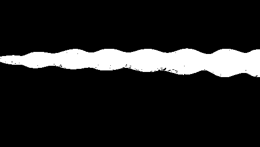
Remark: Applying ColorNegate seems appropriate, but we get good results without it.
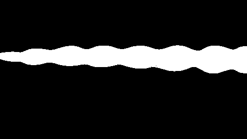
Remove the black spots inside the blade:
img3 = Dilation[img2, 1.2]
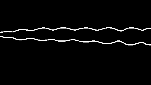
Edge detect and dilate:
img4 = Dilation[EdgeDetect[img3], 1.2]
Extract the edge points and plot them:
lsPoints = Reverse /@ Position[ImageData[img4], 1, 2];
ListPlot[lsPoints]
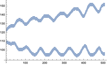
Separate the extracted points (one set for each dagger edge):
lsPoints2 = GatherBy[lsPoints, #[[2]] > 115 &];
ListPlot[lsPoints2]
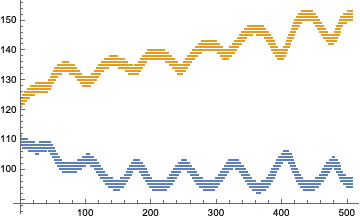
Using FindFormula would have been nice if it worked:
fm = FindFormula[lsPoints2[[1]], TargetFunctions -> {Sin, Cos, Times, Plus}]

ListPlot[fm /@ Range @@ MinMax[Append[lsPoints2[[2]][[All, 1]], 5]]]
We can use Fit and NonLinearFit but then we have to think about appropriate models. It is much easier to use the resource function QuantileRegression. Here is an example:
qrFunc = First@ResourceFunction["QuantileRegression"][lsPoints2[[2]], 30, 0.5];
Show[ListPlot[lsPoints2[[2]], PlotStyle -> Gray], Plot[qrFunc[x], {x, 0, 500}, PlotStyle -> Red]]
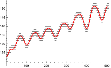
Let us introduce random noise into the dagger-upper-edge points and then find and plot the fitted curves a few times (or five):
lsPoints3 = SortBy[lsPoints2[[2]], First][[1 ;; -1 ;; 3]];
lsQRFuncs = Table[First@ResourceFunction["QuantileRegression"][lsPoints3 + RandomVariate[NormalDistribution[0, 8], Length[lsPoints3]], 30, 0.5], 5];
lsQRFuncs = Map[PiecewiseExpand[#[x]] &, lsQRFuncs];
Show[ListPlot[lsPoints2[[2]], PlotStyle -> GrayLevel[0.7]], Plot[lsQRFuncs, {x, 0, 500}, PlotStyle -> Directive[{AbsoluteThickness[3]}], PerformanceGoal -> "Speed", PlotTheme -> "Scientific", AspectRatio -> 1/3]]
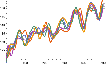
Plot each of the obtained lines separately:
Map[Plot[#, {x, 0, 500}, PlotStyle -> Directive[{Red, AbsoluteThickness[2]}], AspectRatio -> 1/3, PerformanceGoal -> "Speed", PlotTheme -> "Web"] &, lsQRFuncs]

Remark: The wavy curves can be "tuned" by using different number of knots and different random noise distributions



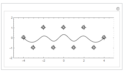



LineIntegralConvolutionPlot, but I have no idea how to adapt it to hair that has overlaps etc. $\endgroup$