3
$\begingroup$

I am trying to plot a phase angle vs. frequency curve numerically for the steady state condition of the following equation

x''[t] + 2 ζ x'[t] + x[t] == Cos[w t]

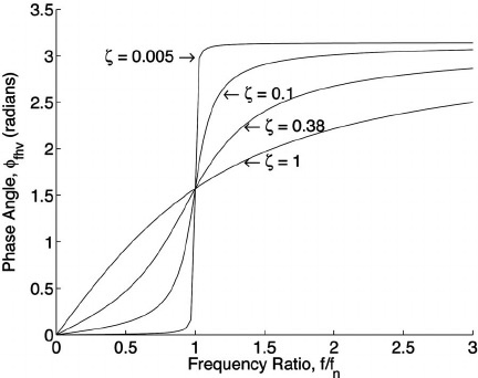
where w is the forcing frequency, and the initial conditions are x[0] == 0, x'[0] == 0. A similar plot is shown here:

sample-plot

$\endgroup$
1
  • 1
    $\begingroup$ Basically you want a Bode plot, right? $\endgroup$
    – codebpr
    Commented Feb 9 at 14:10

2 Answers 2

10
$\begingroup$

Method 1 : Using Bode Plot from signals and systems

One more direct solution can be by making use of Mathematica's inbuilt BodePlot. You just need to find the Transfer function, which can be easily found in your equation by taking the Laplace Transform on both sides of the equation and is given as:

H[s_] := 1/(s^2 + 2 \[Zeta]  s + 1)

Now, use the BodePlot function, just for Phase by this code:

BodePlot[1/(s^2 + 2 (#)  s + 1) & /@ {0.005, 0.1, 0.38, 1}, 
 PlotLayout -> "Phase", 
 PlotLegends -> 
  Placed[LineLegend[{0.005, 0.1, 0.38, 1}, LegendLabel -> "\[Zeta]", 
    LegendFunction -> (Framed[#, RoundingRadius -> 5] &), 
    LegendMargins -> 3], {0.8, 0.7}]]

Which gives you a similar answer as given by @Nasser. You just need to change your units to the ones described in the reference.
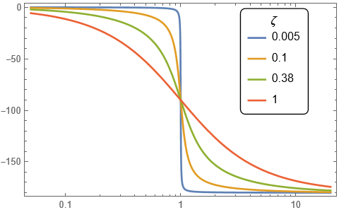
bode-plot

Method 2: Using Direct formula from the theory of vibrations

You can easily find the theory of forced harmonic vibrations in any of the books on mechanical vibrations, like Theory of Vibration with Applications by William Thomson and Theory of Vibration, An Introduction by Ahmed A. Shabana, which directly provides you with the formula for phase angle ($\psi$) in terms of damping factor ($\zeta$) and frequency ratio ($r$) as:

$$ \psi = \tan^{-1} \bigg( \frac{2 r \zeta}{1-r^2} \bigg) $$

Then it's really easy to plot the phase-frequency curve:

\[Psi][\[Zeta]_, r_] := ArcTan[1 - r^2, 2  r  \[Zeta]];

Plot[Evaluate@
  Table[\[Psi][\[Zeta], r], {\[Zeta], {0.005, 0.1, 0.38, 1}}], {r, 0, 
  4}, PlotRange -> {{0, 3}, {0, 3.5}}, AspectRatio -> 1/GoldenRatio, 
 PlotPoints -> 1000, PlotTheme -> {"Scientific", "NeonColor"}, 
 FrameLabel -> {"Frequency ratio \[Rule]", "Phase angle \[Rule]"}, 
 LabelStyle -> {Black, Bold, 15}, 
 PlotLegends -> 
  Placed[SwatchLegend[Automatic, {0.005, 0.1, 0.38, 1}, 
    LegendMarkers -> "Bubble", LegendMarkerSize -> 20, 
    LegendFunction -> (Framed[#, RoundingRadius -> 10, 
        Background -> GrayLevel[0.85]] &), 
    LegendLabel -> "\[Zeta]"], {0.9, 0.25}], ImageSize -> Large]

which gives you the desired plot:
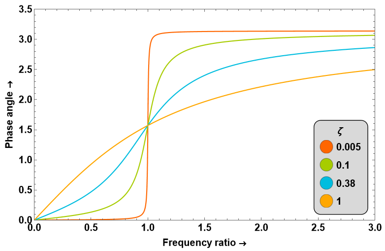
phase-frequency

$\endgroup$
9
  • $\begingroup$ Thankyou for your timely response. If the differential equation is highly nonlinear and it is not possible to take Laplace transform for the differential equation, in that case what can I do or is there any alternative for the same? $\endgroup$
    – Abhishek
    Commented Feb 9 at 16:00
  • $\begingroup$ @Abhishek can you provide me an example for such an equation related to your work? I will try to figure out a way. $\endgroup$
    – codebpr
    Commented Feb 9 at 17:11
  • $\begingroup$ Sure. Here is the equation: x''[T] == (1/\[Epsilon])*((((1 + WE)*(1 + \[Epsilon]*x[T])^(-3*\[Kappa] -1))) - ((1 + \[Epsilon]* x[T])^-1) - (WE*(1 + \[Epsilon]*x[T])^-2) - (4*damping*\[Epsilon]^2*(x'[T])*(1 + (\[Epsilon]* x[T]))^-2) - ((3*\[Epsilon]^2*(x'[T]^2)*(1 + \[Epsilon]*x[T])^-1)/2) - \[Epsilon]^3*f*Sin[T* (w0 + \[Epsilon]^2 w)]) with the initial conditions x[0]=1, x'[0]=0 $\endgroup$
    – Abhishek
    Commented Feb 9 at 17:28
  • $\begingroup$ and the values of the constants are WE=0.2, \[Kappa]=1.4, \[Epsilon]=0.1, and damping=0.03 $\endgroup$
    – Abhishek
    Commented Feb 9 at 17:30
  • 2
    $\begingroup$ @Abhishek, Transfer function is used in frequency domain analysis and that for linear systems only. You can't have it for any nonlinear system unless you linearize it around some point. Nonlinear systems can be chaotic as well and there is no analytic method to solve them. I suggest you post a new question, where you discuss the details of your problem, what have you tried so far and what do you expect as the result, along with related links of your equations on bubble oscillations. Experts on non-linear can then definitely answer that. If you are satisfied, don't forget to accept the answer. $\endgroup$
    – codebpr
    Commented Feb 10 at 18:24
7
$\begingroup$

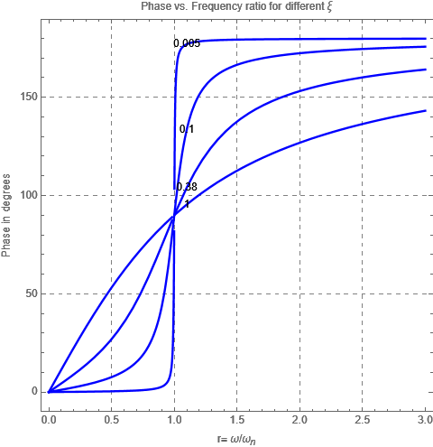
Mathematica graphics

Code

phase[r_, z_] := Module[{t}, t = ArcTan[(2 z  r)/(1 - r^2)];
   If[t < 0, t = t + Pi];
   180/Pi  t];
plotOneZeta[z_, f_] := Module[{r, p1, p2},
   p1 = Plot[f[r, z], {r, 0, 3}, PlotRange -> All, 
     PlotStyle -> Blue];
   p2 = Graphics[Text[z, {1.1, f[1.1, z]}]];
   Show[{p1, p2}]];
p = Map[plotOneZeta[#, phase] &, {.005, 0.1, 0.38, 1}];
Show[p, FrameLabel -> {{"Phase in degrees", 
    None}, {"r= ω/ωn", 
    "Phase vs. Frequency ratio for different ξ"}}, Frame -> True, 
 GridLines -> Automatic, GridLinesStyle -> Dashed, ImageSize -> 400, 
 AspectRatio -> 1]

Use degree for phase not radians. You can easily change that.

ps. I stole the code from this page

$\endgroup$
1
  • 1
    $\begingroup$ Thanks for the response. Is there any direct method to obtain the same plot for highly nonlinear differential equation? $\endgroup$
    – Abhishek
    Commented Feb 9 at 15:58

Your Answer

By clicking “Post Your Answer”, you agree to our terms of service and acknowledge you have read our privacy policy.

Not the answer you're looking for? Browse other questions tagged or ask your own question.