Steady State Numerical Solution of Heat Diffusion Equation in 2D

Question

I'v been trying to solve for the steady state of the heat diffusion equation numerically but I cant seem to get it to work. My code is

pde = D[u[x, y], {x, 2}] + D[u[x, y], {y, 2}] == 0
sol = NDSolve[{pde, u[x, 0] == 100, u[x, 10] == 400, u[0, y] == 0, 
u[10, y] == 0}, u[x, y], {x, 0, 10}, {y, 0, 10}] 

and I get this error

NDSolve::ivone: Boundary values may only be specified for one independent
variable. Initial values may only be specified at one value of the other 
independent variable.

I think It has something to do with there not being an initial value condition, but I don't have one since I'm solving for the steady state. Could anyone please tell me where the above error comes from? Any help would be appreciated. Thanks.

Answer 1

If you have v.10 you can explicitly use the finite element method:

Needs["NDSolve`FEM`"]
mesh = ToElementMesh[Rectangle[{0, 0}, {10, 10}]]
sol = First@NDSolveValue[{Laplacian[w[x, y], {x, y}] == 0,
   DirichletCondition[w[x, y] == 100, y == 0],
   DirichletCondition[w[x, y] == 400, y == 10],
   DirichletCondition[w[x, y] == 0, x == 0],
   DirichletCondition[w[x, y] == 0, x == 10]}, {w}, {x, y} \[Element] mesh];

ContourPlot[sol[x, y], {x, 0, 10}, {y, 0, 10}]

Answer 2

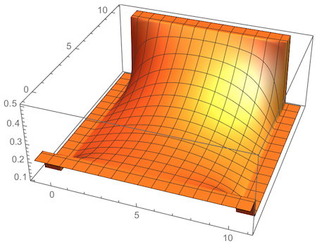
Since you are specifically asking about versions below 10, it may be useful to point out that this problem is equivalent to the electrostatics problem of finding the potential in a region bounded by conductors held at fixed voltages. This can be solved, e.g., with the simple relaxation method I implemented in this answer, where I actually allow for lots of other complications. The potential is solved on a rectangular grid, and the main point was to play around with a graphical method for specifying the boundary conditions. You can apply that method to the question here as follows (I'm first copying the relevant definitions from the lined answer):

defaultGridSize = 120;
step = 
  Compile[{{phi, _Real, 2}, {orig, _Real, 2}, {mask, _Real, 
     2}, {dchiX, _Real, 2}, {dchiY, _Real, 2}}, 
   Module[{f = (RotateRight[phi] + RotateLeft[phi] + 
          RotateRight[phi, {0, 1}] + RotateLeft[phi, {0, 1}])*mask + 
       orig, ex, ey}, 
    ex = (RotateRight[phi, {0, 1}] - RotateLeft[phi, {0, 1}]);
    ey = (RotateRight[phi] - RotateLeft[phi]);
    f - (dchiX*ex + dchiY*ey)*mask]];

iterate = 
  Compile[{{gridArray, _Real, 2}, {originalArray, _Real, 
     2}, {maskArray, _Real, 2}, {dchiX, _Real, 2}, {dchiY, _Real, 
     2}, {tol, _Real}}, 
   FixedPoint[step[#, gridArray, maskArray, dchiX, dchiY] &, 
    originalArray, 100000, 
    SameTest -> (Max@Abs@Flatten[#1 - #2] < tol &)]];

digitize[gr_, n_] := 
  N@ImageData@
    ColorConvert[
     Image[Show[gr, Background -> Black, 
       BaseStyle -> {Antialiasing -> False}], ImageSize -> n], 
     "GrayScale"];

createLandscape[conductors_, chargePlus_, chargeMinus_, 
   suceptibility_, nGrid_] := 
  Module[{gridConductors, gridRho, gridChi, maskList}, 
   gridConductors = digitize[conductors, nGrid];
   maskList = N[1. - Unitize[gridConductors]];
   gridRho = (digitize[chargePlus, nGrid] - 
       digitize[chargeMinus, nGrid])*maskList;
   gridChi = digitize[suceptibility, nGrid]*maskList;
   {gridConductors, gridRho, gridChi, maskList}];

poissonSolver[conductors_, chargePlus_, chargeMinus_, suceptibility_, 
   nGrid_: defaultGridSize, tolerance_: 10^(-6)] := 
  Block[{averagePotential, gridConductors, gridRho, gridChi, gridEps, 
    gridList, maskList, mask4List, dChiYList, dChiXList, 
    initialGrid}, {gridConductors, gridRho, gridChi, maskList} = 
    createLandscape[conductors, chargePlus, chargeMinus, 
     suceptibility, nGrid];
   averagePotential = Mean[Select[Flatten@gridConductors, Positive]];
   initialGrid = averagePotential*maskList + gridConductors;
   gridEps = 1. + gridChi;
   gridList = gridConductors + gridRho/(4.*gridEps);
   mask4List = maskList/4.;
   dChiYList = (RotateLeft[gridChi] - 
       RotateRight[gridChi])/(2. gridEps);
   dChiXList = (RotateLeft[gridChi, {0, 1}] - 
       RotateRight[gridChi, {0, 1}])/(2. gridEps);
   Reverse@
    iterate[gridList, initialGrid, mask4List, dChiXList, dChiYList, 
     tolerance]];

Now for the specific boundary conditions. The region extends from 0 to 10 in both directions, but I need to add some padding on the outside in order to define areas with the desired boundary potential. So the simulation area is the square extending from -1 to 11 in both directions (this is where the figure shows rectangles in various gray shades):

conductors = 
 Graphics[{{GrayLevel[.5], Rectangle[{0, 10}, {10, 11}]},
   {GrayLevel[.1], Rectangle[{10, 0}, {11, 11}]}, {GrayLevel[.2], 
    Rectangle[{-1, -1}, {11, 0}]},
   {GrayLevel[.1], Rectangle[{-1, 0}, {0, 11}]}},
  PlotRangePadding -> 0, ImagePadding -> None]

To explain how I chose the conductor potentials: in my graphical approach, the color black corresponds to the absence of any object. All other potentials are encoded in the grayscale value of the region. This means the value 0 can't be used as a potential, and therefore I shift all potentials by a value 0.1 to make them non-zero. Also, I rescaled all potentials so that they fit into the interval from .1 to 1 that can be directly translated to GrayLevel. This means I have to use the following correspondence between your boundary conditions and mine:

• 0 $\mapsto$ .1
• 100 $\mapsto$ .2
• 400 $\mapsto$ .5.

There is no need to specify any of the other electrostatic quantities, except to define their corresponding graphics objects to be empty. Then I invoke the solver:

chargePlus = 
  Graphics[{}, PlotRange -> (PlotRange /. FullOptions[conductors])];

chargeMinus = 
  Graphics[{}, PlotRange -> (PlotRange /. FullOptions[conductors])];

susceptibility = 
  Graphics[{}, PlotRange -> (PlotRange /. FullOptions[conductors])];

Timing[potential = 
   poissonSolver[conductors, chargePlus, chargeMinus, susceptibility];]

(* ==> {5.65001, Null} *)

ListPlot3D[potential, PlotRange -> All, 
 PlotStyle -> {Orange, Specularity[White, 10]},
  DataRange->{{-1,11},{-1,11}}]

For more details, you may want to consult the link I gave above.