51
$\begingroup$

I am trying to plot a polynomial of degree $29$ on the domain $[0,1]$, with fairly large coefficients:

poly[z_] = -1.1126829840302355` + 113.28783661058498` z - 
9878.742379213338` z^2 + 584715.8646149524` z^3 - 
2.280647160113914`*^7 z^4 + 6.176933520283158`*^8 z^5 - 
1.217581378062843`*^10 z^6 + 1.811582263559531`*^11 z^7 - 
2.0920133095023196`*^12 z^8 + 1.9158620445090305`*^13 z^9 - 
1.414955836879161`*^14 z^10 + 8.539129365981781`*^14 z^11 - 
4.254563022912091`*^15 z^12 + 1.764182366816184`*^16 z^13 - 
6.125080435776876`*^16 z^14 + 1.7883504482275766`*^17 z^15 - 
4.403320010637656`*^17 z^16 + 9.154951756734264`*^17 z^17 - 
1.6068672087698447`*^18 z^18 + 2.3765393965161196`*^18 z^19 - 
2.950846281328122`*^18 z^20 + 3.0579497598096415`*^18 z^21 - 
2.6220913470110597`*^18 z^22 + 1.837651151556163`*^18 z^23 - 
1.0344252684666292`*^18 z^24 + 4.5602474296077024`*^17 z^25 - 
1.5155510563521117`*^17 z^26 + 3.568596763872067`*^16 z^27 - 
5.304183668348243`*^15 z^28 + 3.7404713997980006`*^14 z^29

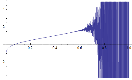
The problem is that when I try to plot the polynomial, all seems fine near 0, but then midway through the unit interval I observe some erratic behaviour as shown below. Can anyone tell me why this is and how I can avoid it?

Plot[{poly[z]}, {z, 0, 1}, WorkingPrecision -> precision]

I would expect the polynomial to be a smooth curve

$\endgroup$
3
  • 7
    $\begingroup$ Have you considered that you're working with a 29th degree polynomial with insanely huge coefficients? It's not surprising to me that you get a plot like that. It may seem "nice" early on, but that's because z^29 (and other high-order terms) is very small near 0. Near approximately 0.85, it rapidly approaches 1. $\endgroup$ Commented Mar 18, 2012 at 2:14
  • 6
    $\begingroup$ @Mithc, I will have to disagree with you. Just because the terms of the ploynomial get large as z goes to 1 does not mean you should expect this type of erratic behaviour. Indeed the polynomial can have no more than 29 real roots! So why you expect a plot like this is beyond me. You should not have voted the question down. I suspect a numerical issue here and was hoping somebody could help me pin it down. $\endgroup$
    – aukie
    Commented Mar 18, 2012 at 3:09
  • 8
    $\begingroup$ It's cancellation error. Per advice in the response, use higher precision and/or rationalize the coefficients. And be sure you know what you are doing in terms of what might comprise an "expected" outcome, because the result might not mean much if the actual coefficients really have error intervals associated with them. $\endgroup$ Commented Mar 19, 2012 at 1:16

4 Answers 4

64
$\begingroup$

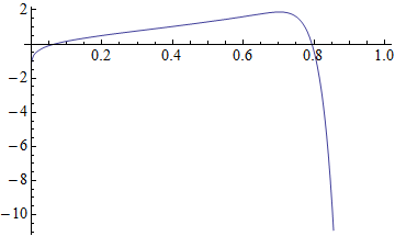
If you Rationalize your real numbers you will be able to use Mathematica's arbitrary precision engine:

poly2 = Rationalize[poly[z], 0];

Plot[poly2, {z, 0, 1}, WorkingPrecision -> 50]
Mathematica graphics


Arbitrary and machine precision

Mathematica has two kinds of numeric calculations: machine precision, and arbitrary precision. Machine precision is fast but is limited to 53 binary (≈16 decimal) digits(1)(2) and may lose precision during a calculation. Mathematica also does not track the precision of a result.

Numbers entered as 1.234 or 1234` are taken to be machine precision.

Arbitrary precision is slower, but Mathematica will track the precision of calculations, often using more calculations as necessary to preserve precision, and print the precision of the result.

Exact values such as 1234 and 1/2 can be used in arbitrary precision calculations. Numbers can also be entered with e.g. 1.234`20 specifying 20 digits of precision, and these will automatically use arbitrary precision if all other values are either exact or arbitrary.

Precision can be checked with the function Precision:

Precision /@ {1.234, 1234`, 1.234`20, 7}
{MachinePrecision, MachinePrecision, 20., ∞ }

Precision can only be preserved if all values in a calculation have at least that precision. Also, arbitrary precision arithmetic may be used with numbers having a precision less than MachinePrecision -- Mathematica will show the true precision of the result.

Precision[1.234 + 7]

Precision[1.234`20 + 1.234`12]
MachinePrecision

12.301

Precision can be set with SetPrecision. It is probably better to use this rather than Rationalize to put numbers into a form that the arbitrary precision engine will use, because the latter will be manufacturing false precision.

Applying this to your problem:

poly3 = SetPrecision[poly[z], 15];

Plot[Evaluate[poly3], {z, 0, 1}, WorkingPrecision -> 50]

During evaluation of In[91]:= Plot::precw: The precision of the argument function <<>> is less than WorkingPrecision (50.`). >>

This is an important warning because it lets you know that your results may not be valid.

See this tutorial for more information about precision. Take time to understand the difference between Mathematica's meanings of Accuracy and Precision.


Recommended reading, a more recent answer from Szabolcs regarding arbitrary precision:


Interval

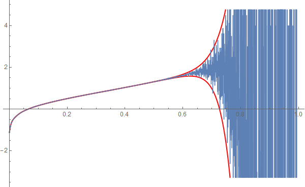
Michael's answer shows the folly of simply doing a Rationalize as I did at the start of this answer. Since questions like this come up often it would be good to have a general solution that is easily applied. I propose this rule using his formula:

machineToInterval = 
  c_Real?MachineNumberQ :> 
    Interval[ {1 - 2^-54, 1 + 2^-54} SetPrecision[c, ∞] ];

This converts any machine numbers into explicit Interval form.

To extract an ordered pair of values from a numeric Interval we merely need First.

poly3 = poly[z] /. machineToInterval;

Plot[{First @ poly3, poly[z]}, {z, 0, 1}
 , WorkingPrecision -> 50
 , PlotStyle -> {{Thick, Red}, ColorData[97][1]}
]
enter image description here

$\endgroup$
4
  • $\begingroup$ @Wizard, Thank you. If possible can you give me some insight into the problem and the solution. $\endgroup$
    – aukie
    Commented Mar 18, 2012 at 3:22
  • 1
    $\begingroup$ @aukie see the updated answer $\endgroup$
    – Mr.Wizard
    Commented Mar 18, 2012 at 12:05
  • 7
    $\begingroup$ To complement this, calculating the polynomial value in Horner form (HornerForm) increases precision somewhat, but not enough. $\endgroup$
    – Szabolcs
    Commented Mar 18, 2012 at 22:26
  • $\begingroup$ @Szabolcs But strangely enough including WorkingPrecision->20 does allow HornerForm to work: Plot[HornerForm[poly[z]] // Evaluate, {z, 0, 1}, WorkingPrecision -> 20] // Quiet. $\endgroup$
    – JimB
    Commented Feb 11, 2022 at 23:42
33
$\begingroup$

Here is another way to look at the OP's plot, which came to me after reading Daniel Lichtblau's comment under the question. His comment is worth emphasizing, which I think the following will show. (Mr.Wizard alludes to the issue in his remark on validity near the end of his answer.)

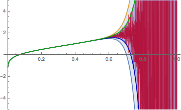
Let's say that machine precision is binary64, which has 53 bits of precision, and the maximum relative rounding error is 2^-53. Let's be a little fuzzy and say that the average error is roughly half that or 2^-54. The we can get almost exactly the envelope of the OP's plot as follows. We can replace the coefficients with ones that are slightly larger and smaller (according with the relative error); since z >= 0, the two resulting polynomials form estimates for the upper and lower bounds on poly[z]. (I'll use a high working precision, as in Mr.Wizard's answer, to compute the bounds precisely.)

Let's show two sets of bounds: bounds is in accordance with the average relative error and will form the envelope of the OP's plot; and absbounds is in accordance with the maximum relative error.

boundsPlot[error_, opts : OptionsPattern[Plot]] := With[{
    polyMin = poly[z] /. c_Real :> (1 - Sign[c] error) SetPrecision[c, Infinity],
    polyMax = poly[z] /. c_Real :> (1 + Sign[c] error) SetPrecision[c, Infinity]},
   Plot[{polyMin, polyMax}, {z, 0, 1}, WorkingPrecision -> 50, Filling -> {1 -> {2}}, opts]
   ];
bounds = boundsPlot[2^-54, PlotStyle -> {Darker@Blue, Darker@Green}, PlotRange -> 5];
absbounds = boundsPlot[2^-53, PlotRange -> 5];

plotOP = Plot[poly[z], {z, 0, 1}, PlotStyle -> {AbsoluteThickness[0.7], Red}, PlotRange -> 5];

Show[plotOP, absbounds, bounds]

Mathematica graphics

A good way to think of floating-point numbers is that they represent an interval of real numbers. At best a floating-point number is an approximation obtained by rounding the true value in an interval to the binary representative. An average error of 2^-54 is about as precise as the coefficients could be if they are thought of as random variables uniformly distributed throughout each interval. The bounds above show the range of likely possible values of poly[z], although occasionally poly[z] exceeds bounds.

The upshot is this: Under the hypothesis that the coefficients are known to MachinePrecision, the OP's original plot more accurately represents what is known about poly[z], than the better-looking high-precision plot. The plot bounds seems to show the likely limits of the plot of the polynomial, under the same hypothesis (although calculating the probability is beyond me). Similarly, the plot absbounds shows absolute bounds on the poly[z]. Under the hypothesis, using absbounds or bounds seems the appropriate way to represent poly[z].

If the error is greater than 2^-53, say, because the coefficients are calculated from scientific measurements with less precision, then one can compute the corresponding bounds.

$\endgroup$
6
  • $\begingroup$ Great analysis. +1 $\endgroup$
    – Mr.Wizard
    Commented Sep 14, 2014 at 0:28
  • $\begingroup$ I forgot that I needed to apply the variation to the mantissa. Correcting that I get a result that matches yours. $\endgroup$
    – Mr.Wizard
    Commented Sep 14, 2014 at 6:11
  • $\begingroup$ Actually it doesn't quite, and I have a guess why. $\endgroup$
    – Mr.Wizard
    Commented Sep 14, 2014 at 6:32
  • $\begingroup$ I am using r_Real :> (Interval[Rationalize[#, 0] + {-1, 1} 2^-54] 10^#2 & @@ MantissaExponent[r]). Is this more or less accurate than your method? $\endgroup$
    – Mr.Wizard
    Commented Sep 14, 2014 at 6:53
  • 3
    $\begingroup$ @Mr.Wizard Ah, I see. I missed that. SetPrecision directly converts the binary representation of a machine real into a rational number with an appropriate 2^n denominator. Rationalize replaces c by the rational number with the smallest denominator within roughly c * $MachineEpsilon of c (e.g. SetPrecision[1./3, Infinity]` vs. Rationalize[1./3, 0]). SetPrecision accurately corresponds to the process I described in my answer. Rationalize does something different but close; I don't think that it is the function to use in this analysis. $\endgroup$
    – Michael E2
    Commented Sep 14, 2014 at 12:30
15
$\begingroup$

Surprisingly enough, converting the polynomial to the Bernstein basis yields a result that Plot[] can stably deal with:

pbconv[poly_, x_] /; PolynomialQ[poly, x] := Module[{bc, n},
                  n = Exponent[poly, x];
                  bc = CoefficientList[poly, x]/Binomial[n, Range[0, n]];
                  Do[bc[[j + 1]] += bc[[j]], {k, n, 1, -1}, {j, k, n}];
                  bc]

pb[z_] = With[{n = Exponent[poly[z], z]}, 
              N[pbconv[SetPrecision[poly[z], ∞], z]] .
              BernsteinBasis[n, Range[0, n], z]]

(The cheating with SetPrecision[] is necessary because, as mentioned in the answer I linked to, the conversion procedure is inherently ill-conditioned.)

A plot:

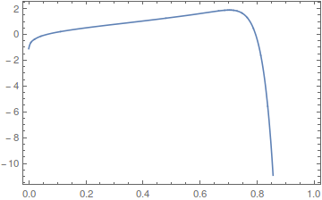
Plot[pb[z], {z, 0, 1}]

look how smooth it got

This suggests that whatever process that generated the original polynomial might have been better reformulated in the Bernstein basis.

$\endgroup$
3
$\begingroup$

Settled complain about my post being "off topic". (My post got complaints about not using a special language thats too expensive for me to buy:"this is a Wolfram Language, not a mathematics, site". I did not pay attention to the brand name in the domain name. I removed the offending post for the reader's benefit.)

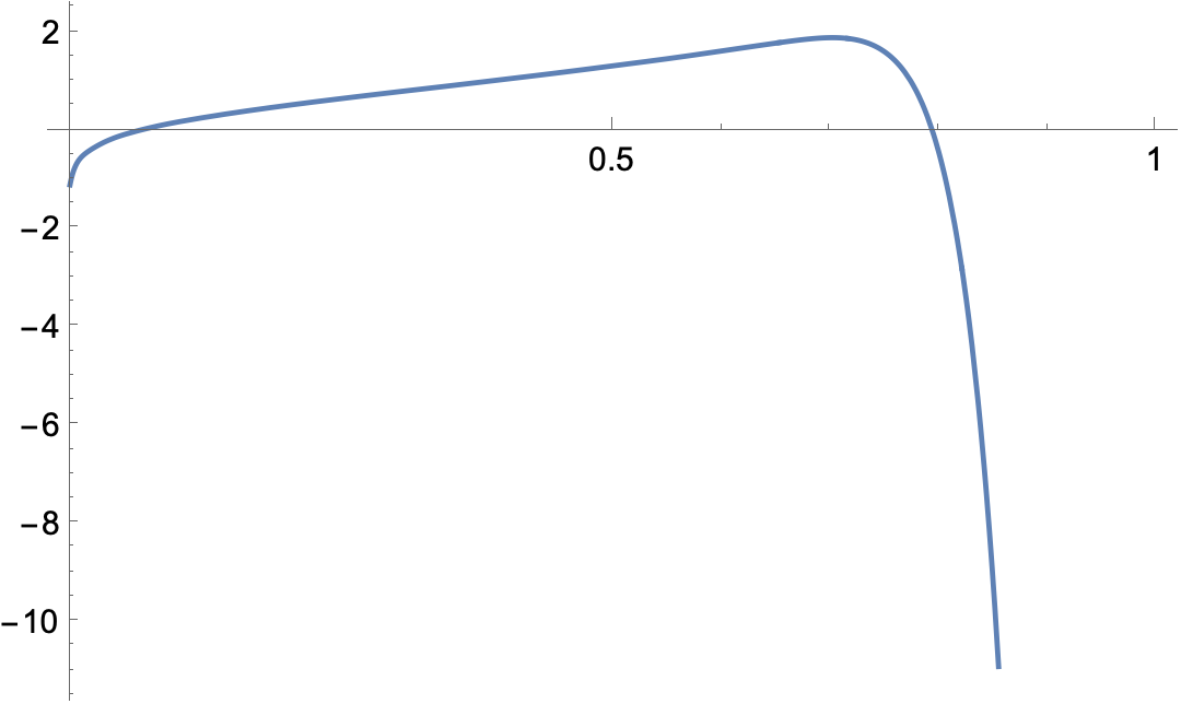
Here is @fischertranscripts's idea in Mathematica code (from @MichaelE2), which idea is to center the expansion at the center of the interval to reduce catastrophic cancellation:

p4 = SetPrecision[poly[z], Infinity] /. z -> y + 4/10 // Expand // N
(*
1.036149520209514` + 2.6409755026207726` y - 
 0.26953631057648186` y^2 + 3.449324571015004` y^3 + 
 338.0294181630971` y^4 - 11.745703101835632` y^5 - 
 43728.76625187574` y^6 - 8023.6344953736` y^7 + 
 2.8981359277591794`*^6 y^8 + 319591.7190295984` y^9 - 
 1.1561838608969387`*^8 y^10 + 1.6950583018096235`*^7 y^11 + 
 2.9997779821296453`*^9 y^12 - 1.5058103605142357`*^9 y^13 - 
 5.259500639613633`*^10 y^14 + 4.791402548859846`*^10 y^15 + 
 6.297914684319244`*^11 y^16 - 8.57877729466455`*^11 y^17 - 
 5.062935150456753`*^12 y^18 + 9.554822737249043`*^12 y^19 + 
 2.5656319594205586`*^13 y^20 - 6.75013786580717`*^13 y^21 - 
 6.66863314102059`*^13 y^22 + 2.924066304682213`*^14 y^23 - 
 1.0628093808994717`*^13 y^24 - 6.905409809370671`*^14 y^25 + 
 5.294845683864764`*^14 y^26 + 5.772127663081625`*^14 y^27 - 
 9.652368445825622`*^14 y^28 + 3.7404713997980006`*^14 (y^29) 
*)

Plot[p4, {y, -0.4, 0.6}, AxesOrigin -> {-0.4, 0}, 
 Ticks -> {Charting`ScaledTicks[{# - 0.4 &, # + 0.4 &}], Automatic}]

enter image description here

$\endgroup$
6
  • 2
    $\begingroup$ Perhaps, you could plot the curve for your transformed polynomial. $\endgroup$
    – bbgodfrey
    Commented Feb 11, 2022 at 10:27
  • $\begingroup$ And show the expansion that gave that particular set of coefficients. $\endgroup$ Commented Feb 11, 2022 at 13:33
  • $\begingroup$ Hard to beat Plot[Evaluate@{poly[z]}, {z, 0, 1}, WorkingPrecision -> precision], for "easy", if you're starting from Plot[{poly[z]}, {z, 0, 1}, WorkingPrecision -> precision] (assuming precision is >20). As this is a Wolfram Language, not a mathematics, site, it would be better to post your solution in WL code. For instance, p4 = SetPrecision[poly[z], Infinity] /. z -> y + 4/10 // Expand // N; Plot[p4, {y, -0.4, 0.6}], which takes 0.159 sec. compared to 0.0167 sec for precision = 20. $\endgroup$
    – Michael E2
    Commented Feb 11, 2022 at 21:37
  • $\begingroup$ It was a pretty good idea though, and it happened to work pretty well. But for someone who does not know or have the tools you used, it's a lot harder than using Mathematica to accomplish the equivalent thing. -- Roll back my edit if you'd rather your answer be deleted. $\endgroup$
    – Michael E2
    Commented Feb 12, 2022 at 2:19
  • $\begingroup$ @fischertranscripts What I meant by "happened" is that the coefficients after the transformation happened to have negligible cancellation error. I think your transformation will reduce it, but does it always make it negligible? $\endgroup$
    – Michael E2
    Commented Feb 12, 2022 at 15:53

Your Answer

By clicking “Post Your Answer”, you agree to our terms of service and acknowledge you have read our privacy policy.

Not the answer you're looking for? Browse other questions tagged or ask your own question.