4
$\begingroup$

I have a similar problem to Funny behaviour when plotting a polynomial of high degree and large coefficients. However, the thing being evaluated is not just a polynomial, but a dot product of some coefficients with a list of polynomials.

(The back story is that I want to distort a sine random variable so that it has an approximate Laplace distribution. I am doing this by approximating the nonlinear mapping with a Chebyshev approximation. This has the cool property that if I use a maxN-th order Chebyshev series then there are only maxN harmonics of the sine wave. If the exact mapping is used, there are an infinite number of harmonics.)

The dot product (coefficients times Chebyshev polynomials) begins to become inaccurate (blow up, oscillate like crazy, whatever) near $\pm 1$ for maxN greater than the mid-$40$s. I've tried the Rationalize function on the coefficients--the polynomial coefficients are all integers--but to no avail.

Here is what I've tried. I have included the exact mapping for comparison to the Chebyshev approximation. (Mathematica told me that this involves the SinIntegral so I have hard-coded that into the definition.) The mapping has odd symmetry about the origin so even-order coefficients are zero.

FLaplaceInverse[x_, β_] := 
  Piecewise[{{β Log[2 x], x < 1/2}, {-β Log[2 - 2 x], 
     x >= 1/2}}];
FSine[x_, b_] := (π + 2 ArcSin[x/b])/(2 π);
CompositeSineLaplace[x_] := FLaplaceInverse[FSine[x, 1], 1];
maxN = 49;
chebCoeffList = 
  Table[If[EvenQ[n], 0, 
    N[(4 SinIntegral[(n π)/2])/(n π), 100]], {n, 0, maxN}];
rChebCoeffList = Rationalize[chebCoeffList, 0];
chebPolyList = 
  Table[If[EvenQ[n], 0, ChebyshevT[n, x]], {n, 0, maxN}];
plotBoth = 
  Plot[{CompositeSineLaplace[x], 
    rChebCoeffList.chebPolyList} , {x, -1, 1}, PlotRange -> Automatic,
    ImageSize -> Medium];
plotDiff = 
  Plot[Evaluate[
    CompositeSineLaplace[x] - chebCoeffList.chebPolyList] , {x, -1, 
    1}, PlotRange -> Automatic, ImageSize -> Medium];
chebCoeffsWithOrder = 
  Transpose[{Table[n - 1, {n, Length[chebCoeffList]}], chebCoeffList}];
plotCoeffs = 
  ListPlot[chebCoeffsWithOrder, PlotRange -> All, ImageSize -> Medium];
{plotBoth, plotDiff, plotCoeffs}

The Plot functions give this for maxN = 49.

Chebyshev approx and target function, difference, and the Chebyshev coefficients

$\endgroup$
10
  • 1
    $\begingroup$ It is nice to use the Chebyshev polynomial expansion fo this purpose. However, you are in effect converting back to the ill-conditioned monomial basis here. Why not use Clenshaw? Also, you are wasting effort by not exploiting the oddness of your function; there are identities that only require you to retain the odd terms. $\endgroup$ Commented Aug 1, 2015 at 5:05
  • $\begingroup$ For the time being: try cranking up WorkingPrecision. $\endgroup$ Commented Aug 1, 2015 at 5:05
  • $\begingroup$ Numerical Recipes as well as GNU Scientific Library incorporate Clenshaw's method; I have been using the Numerical Recipes code for a while until I noticed something weird. The NR guys say, compute more Chebyshev coefficients than you need, say M, then just truncate to how many you want, say N < M. The assumption is that the truncated terms will cause a negligible error. However, I found that if I compute M1 then M2 terms and then truncate each time to N terms, the N terms are different for the two cases. I attribute this either to slow convergence to -+infinity at ±1 or my coding error to Ada $\endgroup$
    – Jerry
    Commented Aug 1, 2015 at 5:35
  • $\begingroup$ Hmm… if I find time later I might investigate this (unless somebody beats me to it). Re: NR, they gave the identities for evaluating an odd Chebyshev series efficiently IIRC. Use them! $\endgroup$ Commented Aug 1, 2015 at 5:40
  • $\begingroup$ By suggesting that I increase WorkingPrecision I gather that you mean, add it to the Plot statement. I don't think this will help—anyway, I tried with value of 100 with no change in the plots. $\endgroup$
    – Jerry
    Commented Aug 3, 2015 at 9:49

1 Answer 1

5
$\begingroup$

To resolve this:

Compare

Plot[chebCoeffList.chebPolyList, {x, -1, 1}]

with

Plot[chebCoeffList.Table[If[EvenQ[n], 0, ChebyshevT[n, x]], {n, 0, maxN}],
     {x, -1, 1}]

spot the difference

The blowup seen in the first plot is, as noted, due to the fact that chebPolyList is already converted automatically to the monomial basis, which is terribly ill-conditioned for numerical evaluations of this sort. In contrast, the evaluation in the second one did not involve this conversion; that is, ChebyshevT[] was directly evaluated at the inexact numbers fed to it by Plot[]. Setting WorkingPrecision to a higher value in the first plot can stave off this ill-conditioning, but at the expense of increased effort.


As also noted in the comments, a more efficient way of proceeding would be to use the Clenshaw recurrence to evaluate your Chebyshev series. This has to be modified a bit to exploit the oddness of your function. Thus,

cheboddval[c_?VectorQ, x_] := 
           Module[{n = Length[c], u, v, w, y = 4 x^2 - 2}, 
                  u = c[[n - 1]] + y (v = c[[n]]);
                  Do[w = v; v = u; u = c[[k]] + y v - w, {k, n - 2, 2, -1}];
                  x (c[[1]] + (y - 1) u - v)]

Let's generate your coefficients without the zeroes taking up space:

cc = Table[N[(4 SinIntegral[n π/2])/(n π), 50], {n, 1, maxN, 2}];

Now, the plot:

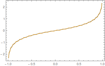
Plot[{CompositeSineLaplace[x], cheboddval[cc, x]}, {x, -1, 1}]

only the tiny wiggles distinguish the two

$\endgroup$

Your Answer

By clicking “Post Your Answer”, you agree to our terms of service and acknowledge you have read our privacy policy.

Not the answer you're looking for? Browse other questions tagged or ask your own question.