Accuracy of Chebyshev Interpolation

Question

I have been looking at how to interpolate a function using Chebyshev polynomials. There are several good posts such as this one by Michael E2 and this one by J. M. There is also an example in the help for FourierDCT. By studying these posts I have assembled a module that does interpolation of a function.

ClearAll[ChebInterpolation];
ChebInterpolation::usage = 
  "ChebInterpolation[f,{xmin,xmax},prec,n] developes an interpolation \
of the function f in the interval [xmin, xmax] based on n Chebyshev \
functions calculated with a precision prec. f must be a pure \
function. ";
ChebInterpolation[f_, {xmin_, xmax_}, prec_, n_] := 
 Module[{nodes, coeff, c},
  nodes = 
   Rescale[N[Cos[Pi Range[0, n]/n], prec], {-1, 1}, {xmin, xmax}];
  coeff = Sqrt[2/n] FourierDCT[f /@ nodes, 1];
  coeff[[{1, -1}]] /= 2;
  c = Compile[{x}, 
    coeff.Table[Cos[(m - 1) ArcCos[x]], {m, Length@coeff}]];
  With[{w = c}, w[Rescale[#, {xmin, xmax}, {-1, 1}]] &]
  ]

With this module I have to supply a precision (prec) and the number of Chebyshev polynomials (n) to use. My question is how to automate finding these two parameters.

I use the module like this. First define a function and the interval within which it will be approximated.

f = BesselJ[1, #^(3/2)] Sin[#] &;
{xmin, xmax} = {25, 35};
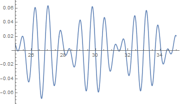
Plot[f[x], {x, xmin, xmax}]

Now we run the module to calculate the interpolation function and plot the result.

fint = ChebInterpolation[f, {xmin, xmax}, 25, 85];
Plot[fint[x], {x, xmin, xmax}]

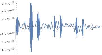
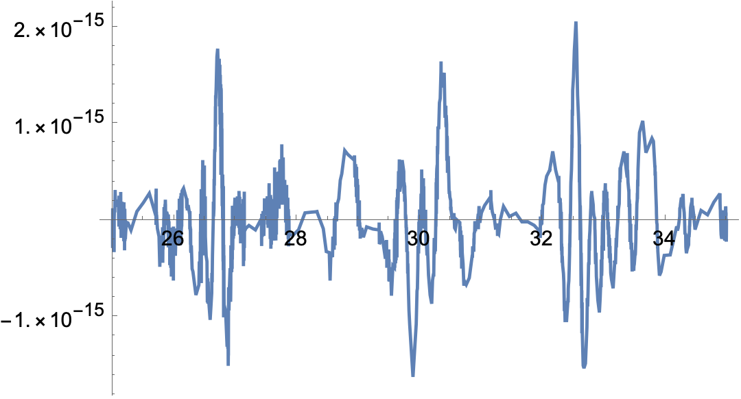
The plot looks very similar and to check the accuracy we can look at the error

Plot[fint[x] - f[x], {x, xmin, xmax}, WorkingPrecision -> 100, 
 PlotRange -> All, PlotPoints -> 100]

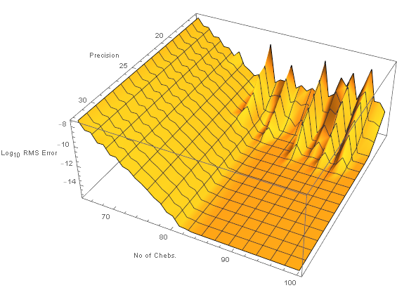
As can be seen the error is small. The parameters in the interpolation were a precision of 25 and 85 Chebyshev polynomials. I used these values by looking at various alternatives. The following calculation determines the log of the RMS error between the exact function and the approximate function for a range of precisions and number of polynomials.

 errs = Table[fint = ChebInterpolation[f, {xmin, xmax}, prec, n];
   e = Table[fint[x] - f[x], {x, xmin, xmax, (xmax - xmin)/100}];
   {prec, n, Log[10, RootMeanSquare[e]]},
   {n, 65, 100}, {prec, 16, 32}];
ListPlot3D[Flatten[errs, 1], PlotRange -> All, 
 AxesLabel -> {"Precision", "No of Chebs.", 
   "\!\(\*SubscriptBox[\(Log\), \(10\)]\) RMS Error"}]

A floor is reached when the precision is about 25 and the number of polynomials is 85.

Question 1: Is my module a good approach or can it be improved?

Question 2: Is looking at the errors in the above plot a robust way of finding the required precision and number of polynomials? If yes, what would be a good way of automating this?

Answer 1

Since we're compiling at the end, doing everything in machine precision seemed okay. We need some cushion for the stopping criterion, since ordinary roundoff error might make achieving a relative error of $MachineEpsilon impossible. I chose a factor of 10, which might not be high enough in every case.

If we think of the order-$n$ Chebyshev points as the $x$ coordinates of $n+1$ points equispaced around the upper half of the unit circle beginning and ending at the endpoints, then to get the order-$2n$ points, we need only bisect each arc. We can add the function values at the new points to the function values at the old points with Riffle[]. Hence we can recursively bisect the half circle until the desired precision is reached.

Since the Chebyshev polynomials satisfy $-1 \le T_j(x) \le 1$ for $-1 \le x \le 1$, the error of truncating the Chebyshev series at order $n$ is bounded by $$\sum_{j=n+1}^\infty |c_j|\,$$ where $c_j$ are the Chebyshev coefficients. For an analytic function, the coefficients decrease geometrically, and the last coefficient $|c_n|$ can be expected to be bound the error, except that any particular coefficient can potentially have any value (just add $a\,T_j(x)$ to your function and you increase the $j$-th coefficient by an arbitrary amount $a$). But this is rare. In practice there's one common such snafu, namely an even or an odd function. If you take the maximium of the last few coefficients (at least two), you can avoid all but the most exceptional problems.

ClearAll[ChebInterpolation];
ChebInterpolation::usage = 
  "ChebInterpolation[f,{xmin,xmax},prec,n] developes an interpolation \
of the function f in the interval [xmin, xmax] based on n Chebyshev \
functions calculated with a precision prec. f must be a pure \
function. ";
ChebInterpolation[f_, {xmin_, xmax_}, prec_] := Module[{nodes, coeff, c
   , n = 8, y, ynew, error = Infinity, tol, len, sum, abscc, maxcc},
  
  (* Need cushion for ordinary roundoff error *)
  tol = Max[10.^-prec, 10*$MachineEpsilon];
  nodes = Rescale[N[Cos[Pi Range[0, n]/n]], {-1, 1}, {xmin, xmax}];
  y = f /@ nodes;
  While[
   error > tol && n < 2^24,
   n = 2*n;
   nodes = Rescale[N[Cos[Pi Range[1, n, 2]/n]], {-1, 1}, {xmin, xmax}];
   ynew = f /@ nodes;
   y = Riffle[y, ynew]; (* riffle new func vals *)
   coeff = Sqrt[2/n] FourierDCT[y, 1];
   coeff[[{1, -1}]] /= 2;
   (* error estimate, save abs/max cc for after *)
   abscc = Abs@coeff;
   maxcc = Max@abscc;
   error = Max[abscc[[-3 ;;]]]/maxcc (* use last 3 coeff to est. 
   error *)
   ];
  (* trim coeffs *)
  sum = 0;
  len = LengthWhile[Reverse@abscc, (sum += #) <= tol*maxcc &];
  coeff = If[TrueQ[len > 1], Drop[coeff, -len], coeff];
  (*foo=coeff;*)
  c = Compile[{x},
    Block[{cc = coeff},
     cc . Table[Cos[(m - 1) ArcCos[x]], {m, Length@cc}]
     ], CompilationOptions -> {"InlineExternalDefinitions" -> True}];
  With[{w = c}, w[Rescale[#, {xmin, xmax}, {-1, 1}]] &]]

Example:

f = BesselJ[1, #^(3/2)] Sin[#] &;
{xmin, xmax} = {25, 35};
fint = ChebInterpolation[f, {xmin, xmax}, 25];
Plot[fint[x] - f[x], {x, xmin, xmax}, WorkingPrecision -> 100, 
 PlotRange -> All, PlotPoints -> 100]

Another example (precision goal = 8):

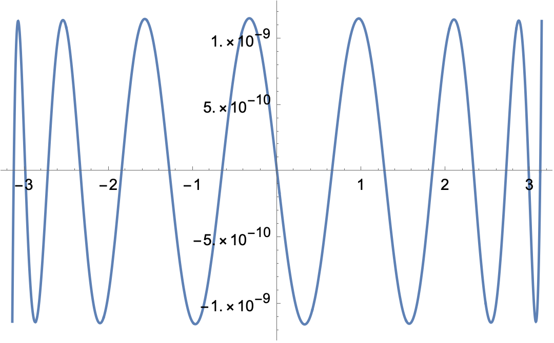
ff = ChebInterpolation[Sin, {-Pi, Pi}, 8];
Plot[ff[x] - Sin[x], {x, -Pi, Pi}]

Looks pretty close to the minimax approximation!