Use NMinimize instead of FindFit for constrained search (of coefficients)

Question

(My problem is more complex, but let us formulate it through this example)

I am trying to find the best polynomial approximation to the following function

f[x_]:=Exp[x]^(1/2) + 2 - Exp[x] + x^5     

through a polynomial (of an arbitrary degree) which would be non-increasing and "best approximation" means in the uniform distance on the interval [0, 1]

I have been trying to implement this with Mathematica, using NMinimize by just taking the code

g[x_]:=a x^2+b x + c

dis[a_, b_, c_] := 
Max[Abs[f[x]-g[x]]]

NMinimize[{dis[a,b,c], 0<=x<=1, 2xa + b <=0 },{a,b,c}]

The first part 0<=x<=1 is the restriction that I care only about for x in [0,1], the second (2xa + b <=0 ) is the restriction that polynomial is non-increasing.

However I get the error that

"The following constraints are not valid: {b+2 a x<=0, 0<=x<=1}. Constraints should be equalities, inequalities, or domain specifications involving the variables"

I mean I cannot use "FindFit" because there is no possibility to constrain the solution (i.e. the structure of the polynomial), nor that I am interested only in the domain $x\in[0,1]$

I would appreciate any thoughts on this, how to proceed...!

PS: In fact I would be quite interested to know how more generally one could incorporate constraints on the solution in terms of the fitting function (e.g. that it also integrates up to a given fixed number)

Answer 1

One approach to this kind of problems is to discretize the continuous domain to a finite (but sufficiently large) number of (not necessarily equispaced) samples and then approximate the original problem on this grid. The resulting formulation is a linear programming problem for which efficient solvers are available.

f[x_] := Exp[x]^(1/2) + 2 - Exp[x] + x^5;

l = 5000; (*number of samples of the [0,1] interval*)
xRange = Range[0., 1., 1./(l - 1)]; (*grid points*)

(*auxiliary matrix; note that {a,b,c}.mA is ax^2+bx+c evaluated on the grid points*) 
mA = {xRange^2, xRange, Table[1., {l}]};  

(*auxiliary matrix; note that {a,b,c}.mB is the derivative of ax^2+bx+c evaluated on the grid points*)
mB = {2 xRange, Table[1., {l}]};

sol = (* note introduction of an additional optimization variable delta *)
FindMinimum[{delta, 
       And @@ Thread[-delta <= {a, b, c}.mA - f[xRange] <= delta] && 
        And @@ Thread[{a, b}.mB <= 0]}, {delta, a, b, c}]

{0.181843, {delta -> 0.181843, a -> 0.0695606, b -> -0.139121, 
  c -> 1.81816}}

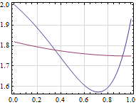
Plot[{f[x], Evaluate[a x^2 + b x + c /. sol[[2]]]}, {x, 0, 1}]

The optimal polynomial approximation in this case is pretty far from close to the actual function due to the non-increasing constraint. Actually, generalizing this approach to larger order polynomials shows that the approximation gets only slightly better. Of course, removing this constraint results in much better approximations that rapidly converge to the actual function with increasing order.

Answer 2

I have tried to implement all advices, but somehow it is still does not work. Here is the code. I must have been missing something gravely...

ClearAll[a, b, c, x, g4, f4, dis]
g4[x_?NumericQ] := a ChebyshevT[2, x] + b  ChebyshevT[4, x]
f4[x_?NumericQ] := Exp[x]^(1/2) + 2 - Exp[x] + x^5
dis[a_?NumericQ, b_?NumericQ, c_?NumericQ, x_] := 
Norm[f4[x] - g4[x], Infinity]
NMinimize[{dis[a, b, c] && 0 <= x <= 1 && 2 x a + b <= 0}, {a, b, c}]

The problem is that I do not have a feeling for the role of NumericQ. I would appreciate any corrections.

Answer 3

The problem that you presented can be solved using FindFit.

You are trying to fit the actual function

f[x_] := Exp[x]^(1/2) + 2 - Exp[x] + x^5

in the range zero to one with a quadratic.

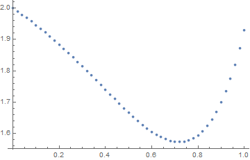
First step is to generate the data. Creating it within the range 0 to 1 satisfies the fist constraint.

data = Table[{x, f[x]}, {x, 0, 1, 0.02}];
ListPlot[data]

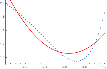
First we will solve it with no additional constraints

sol = FindFit[data, a x^2 + b x + c, {a, b, c}, x]

(* {a -> 1.12792, b -> -1.44246, c -> 2.09175} *)

and then plot and compare it to the original

Show[
 ListPlot[data],
 Plot[Evaluate[a x^2 + b x + c /. sol], {x, 0, 1}, PlotStyle -> Red]
 ]

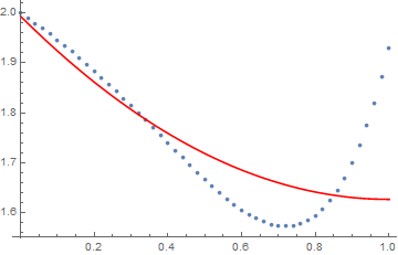
Now we will apply the constraint. One is not allowed to use 2 x a + b <= 0 as it contains the variable. Rather if we look at the constraint and the range we see that the most stringest case is when x=1.

So the new problem with the constraint becomes

sol2 = FindFit[data, {a x^2 + b x + c, 2 a + b <= 0},
                     {{a, 0.5}, {b, -1}, {c, 2}}, x]

(* {a -> 0.367225, b -> -0.734451, c -> 1.99384} *)

and the comparison

Show[
 ListPlot[data],
 Plot[Evaluate[a x^2 + b x + c /. sol2], {x, 0, 1}, PlotStyle -> Red]
 ]