The correct way to linearize colorspace before resizing, blurring etc

Question

There was an interesting discussion on MathGroup dealing with the fact that image-processing functions in Mathematica (and many other software, including Adobe Photoshop) work with RGB, Grayscale etc. intensity values as if they would be linear and additive while in fact these values are powers of the physical intensity values and consequently must be linearized before making additive operations on them. This topic is expanded in the linked article where examples of incorrect default image resizing and blurring are given along with the general explanation of the correct algorithm and images generated with it.

Matthias Odisio (Wolfram Research) replied:

This genuine issue will be properly addressed in a future release of Mathematica.

So, Mathematica 9 is released. But I cannot find any example in the Documentation on how to linearize a colorspace correctly. Obviously, the linearization algorithm must depend on the colorspace used.

The question is: is there efficient and straightforward way to linearize a colorspace in Mathematica correctly?

UPDATE

Here is an excerpt from the documentation for Adobe After Effects which highlights some benefits of linear color space:

By performing operations in a linear color space, you can prevent certain edge and halo artifacts, such as the fringing that appears when high-contrast, saturated colors are blended together. Many color operations benefit from working in a linear color space, including those operations involved in image resampling, blending between layers with blending modes, motion blur, and anti-aliasing.

<...>

Note: A linearized working color space works best with higher color depths—16 bpc and 32 bpc—and is not recommended for 8-bpc color.

Also, good explanation of the difference between linear RGB and sRGB color spaces can be found here.

Answer 1

Here is my attempt to figure out how the correct colorspace linearization should be made. I used specially designed test images by Eric Brasseur for comparison of two colorspace linearization algorithms. The first algorithm is just an implementation of the corresponding formulae from the Specification of sRGB made by Jari Paljakka who started the discussion on MathGroups. This algorithm does not take into acount the alpha channel (and probably will work incorrectly with it). The second algorithm utilizes new image processing functionality of Mathematica 9: the support of colorprofiles.

Both algorithms assume that the input image is in the sRGB colorspace which is the most commonly-used color space and also is the standard default color space for the Internet. More than 90% of all images in the Internet are sRGB-encoded.

The problem with the sRGB colorspace is that it does not have pure gamma curve and hence cannot be correctly linearized just by applying gamma to RGB values. But there is a pure gamma based colorspace: Adobe RGB 1998. So I decided to convert an image to Adobe RGB 1998, then linearize the colorspace by applying gamma using ImageAdjust, resize it with ImageResize (which operates under the assumption of linearity for the pixel data), then apply ImageAdjust with inverse gamma of Adobe RGB 1998 and finally convert from Adobe RGB 1998 to sRGB.

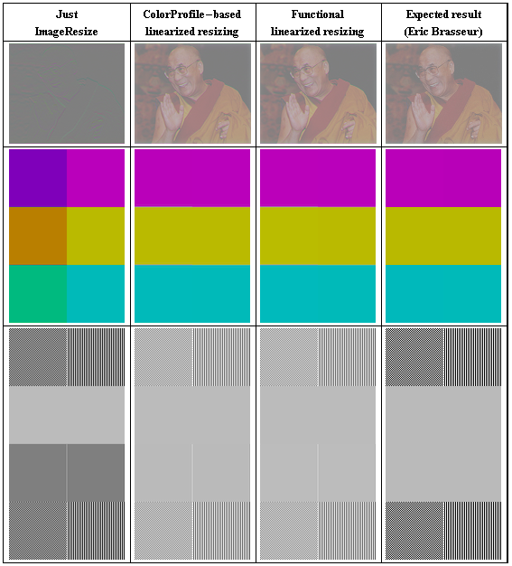
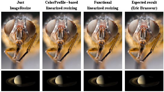
Here is a comparison of the results (these screenshots should be seen in original size with 100% resolution; the code follows):

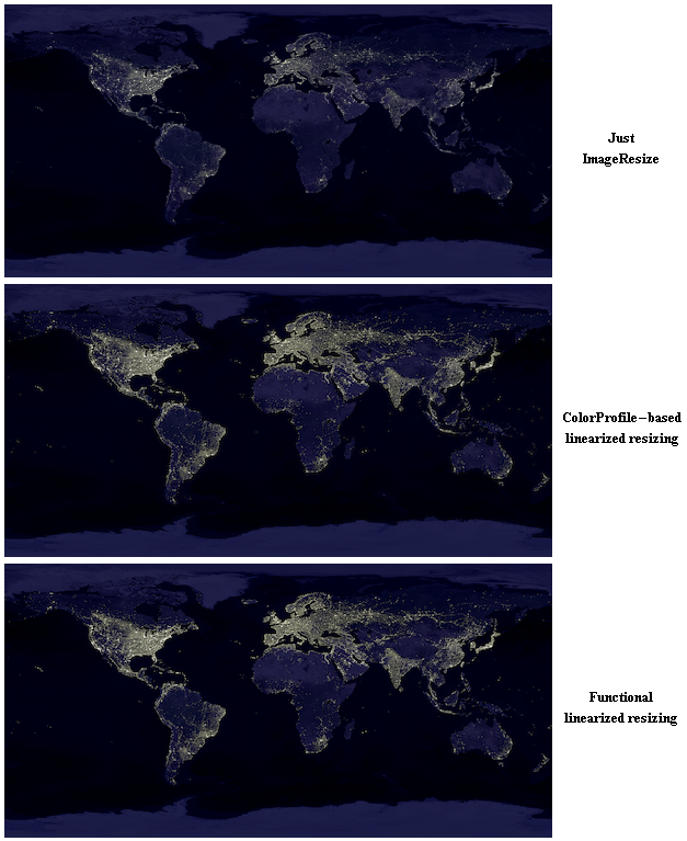
The NASA image "Earth's City Lights" is a very extreme case where non-linear colorspace effects have a big impact on the results of resizing the image (reference from here):

(*Color profile based approach*)
(*The AdobeRGB1998.icc profile is from \
http://www.adobe.com/digitalimag/adobergb.html*)
adobeRGB1998 = Import["AdobeRGB1998.icc"];
(*http://scarse.sourceforge.net/goodies/profiles/*)
sRGB = Import[
   "http://scarse.sourceforge.net/goodies/profiles/spaces/sRGB.icm"];
sRGB2Linear[sRGBimg_Image] := 
 ImageAdjust[
  ColorConvert[
   Image[sRGBimg, "Real",(*ColorSpace->sRGB,*)Interleaving -> True], 
   sRGB -> adobeRGB1998], {0, 0, 563/256}]
linear2sRGB[linearRGB_Image] := 
 ColorConvert[
  Image[ImageAdjust[linearRGB, {0, 0, 256/563}], 
   Interleaving -> True], adobeRGB1998 -> sRGB]
linearResize[sRGBimg_Image, scaling_] := 
 linear2sRGB[ImageResize[sRGB2Linear[sRGBimg], scaling]]
linearBlur[sRGBimg_Image, r_] := 
 linear2sRGB[Blur[sRGB2Linear[sRGBimg], r]]
linear2Grayscale[sRGBimg_Image] := 
 ImageAdjust[
  ColorConvert[sRGB2Linear[sRGBimg], "Grayscale"], {0, 0, 256/563}]


(*functional approach*)
srgb2linear = 
  Compile[{{Csrgb, _Real, 1}}, 
   With[{α = 0.055}, 
    Table[Piecewise[{{C/12.92, 
        C <= 0.04045}, {((C + α)/(1 + α))^2.4, 
        C > 0.04045}}], {C, Csrgb}]], RuntimeAttributes -> {Listable}];
linear2srgb = 
  Compile[{{Clinear, _Real, 1}}, 
   With[{α = 0.055}, 
    Table[Piecewise[{{12.92*C, 
        C <= 0.0031308}, {(1 + α)*C^(1/2.4) - α, 
        C > 0.0031308}}], {C, Clinear}]], 
   RuntimeAttributes -> {Listable}];
linearresize[sRGBimg_Image, scaling_] := 
 Image[linear2srgb[
   ImageData[
    ImageResize[
     Image[srgb2linear[
       ImageData[ColorConvert[Image[sRGBimg, "Real"], "RGB"], 
        Interleaving -> True]], ColorSpace -> "RGB"], scaling], 
    Interleaving -> True]], ColorSpace -> "RGB"]
linearblur[sRGBimg_Image, r_] := 
 Image[linear2srgb[
   ImageData[
    Blur[Image[
      srgb2linear[
       ImageData[ColorConvert[Image[sRGBimg, "Real"], "RGB"], 
        Interleaving -> True]], ColorSpace -> "RGB"], r], 
    Interleaving -> True]], ColorSpace -> "RGB"]
linear2grayscale[sRGBimg_Image] := 
 Image[linear2srgb[
   ImageData[
    ColorConvert[
     Image[srgb2linear[
       ImageData[ColorConvert[Image[sRGBimg, "Real"], "RGB"], 
        Interleaving -> True]], ColorSpace -> "RGB"], "Grayscale"], 
    Interleaving -> True]]]


(*comparison*)
testImages = 
  Import /@ \
{"http://www.4p8.com/eric.brasseur/gamma_dalai_lama_gray.jpg", 
    "http://www.4p8.com/eric.brasseur/gamma_colors.jpg", 
    "http://www.4p8.com/eric.brasseur/gamma_2.2.jpg"};
testImages[[3]] = ImageRotate[testImages[[3]]];
correctResults = 
  Import /@ \
{"http://www.4p8.com/eric.brasseur/gamma_dalai_lama_gray_good.jpg", 
    "http://www.4p8.com/eric.brasseur/gamma_colors_good.jpg", 
    "http://www.4p8.com/eric.brasseur/gamma_good_2.2.jpg"};
correctResults[[3]] = ImageRotate[correctResults[[3]]];
fullSizeFix = 
  Style[Image[#, Magnification -> 1], Magnification -> 1] &;
correctResults = fullSizeFix /@ correctResults;
Grid[Prepend[
  Join[Map[fullSizeFix, {ImageResize[#, Scaled[1/2]], 
       linearResize[#, Scaled[1/2]], linearresize[#, Scaled[1/2]]} & /@
      testImages, {2}], List /@ correctResults, 2], 
  Style[#, Bold, FontFamily -> "Times", 
     TextAlignment -> Center] & /@ {"Just\nImageResize", 
    "ColorProfile-based\nlinearized resizing", 
    "Functional\nlinearized resizing", 
    "Expected result\n(Eric Brasseur)"}], Frame -> All]


calliphora = 
  Import["http://upload.wikimedia.org/wikipedia/commons/8/85/\
Calliphora_sp_Portrait.jpg"];
calliphoraCorrect = 
  Import["http://www.4p8.com/eric.brasseur/gamma_calliphora_sp_\
portrait.1.jpg"];
calliphoraSize = ImageDimensions[calliphoraCorrect];
saturn = Import[
   "http://photojournal.jpl.nasa.gov/jpegMod/PIA11667_modest.jpg"];
saturnCorrect = 
  Import["http://www.4p8.com/eric.brasseur/gamma_388135main_pia11667.\
1.jpg"];
saturnSize = ImageDimensions[saturnCorrect];
Grid[{Style[#, Bold, FontFamily -> "Times", 
     TextAlignment -> Center] & /@ {"Just\nImageResize", 
    "ColorProfile-based\nlinearized resizing", 
    "Functional\nlinearized resizing", 
    "Expected result\n(Eric Brasseur)"}, 
  fullSizeFix /@ {ImageResize[calliphora, calliphoraSize], 
    linearResize[calliphora, calliphoraSize], 
    linearresize[calliphora, calliphoraSize], calliphoraCorrect},
  fullSizeFix /@ {ImageResize[saturn, saturnSize], 
    linearResize[saturn, saturnSize], 
    linearresize[saturn, saturnSize], saturnCorrect}}]

Grid[{Style[#, Bold, FontFamily -> "Times", 
     TextAlignment -> Center] & /@ {"Just\nBlur[#,2]&", 
    "ColorProfile-based\nlinearized blur", 
    "Functional\nlinearized blur", 
    "Expected result\n(Eric Brasseur)"}, 
  fullSizeFix /@ {Blur[testImages[[1]], 2], 
    linearBlur[testImages[[1]], 2], linearblur[testImages[[1]], 2], 
    Import["http://www.4p8.com/eric.brasseur/gamma_dalai_lama_gray_\
blurred.1.jpg"]}}]


gamma4 = Import[
   "http://www.4p8.com/eric.brasseur/gamma_color_to_grayscale_start.\
jpg"];
Grid[{Style[#, Bold, FontFamily -> "Times", 
     TextAlignment -> 
      Center] & /@ {"Just\nColorConvert[#,\"Grayscale\"]&", 
    "ColorProfile-based\nlinearization", "Functional\nlinearization", 
    "Expected result\n(Eric Brasseur)"}, 
  fullSizeFix /@ {ColorConvert[gamma4, "Grayscale"], 
    linear2Grayscale[gamma4], linear2grayscale[gamma4], 
    Import["http://www.4p8.com/eric.brasseur/gamma_color_to_grayscale_\
good.jpg"]}}]


earthLights = 
  Import["http://eoimages.gsfc.nasa.gov/ve//1438/earth_lights_4800.\
tif"];
fullSizeFix = 
  Style[Image[#, Magnification -> 1], Magnification -> 1] &;
Grid[{fullSizeFix /@ {ImageResize[earthLights, 500], 
     linearResize[earthLights, 500], linearresize[earthLights, 500]}, 
   Style[#, Bold, FontFamily -> "Times", 
      TextAlignment -> Center] & /@ {"Just\nImageResize", 
     "ColorProfile-based\nlinearized resizing", 
     "Functional\nlinearized resizing"}
   } // Transpose]

Answer 2

It is arbitrary to assign a color space to data that do not have one attached to them.

What about using "XYZ" if one is looking for a linear color space?

i = Import@"http://www.4p8.com/eric.brasseur/gamma_dalai_lama_gray.jpg";
ColorConvert[i, "XYZ"] // ImageResize[#, Scaled[1/2]] & // 
ColorConvert[#, "RGB"] &