8
$\begingroup$

How do I plot an ParametricPlot with the x-axis using an logarithmic scale? Since I need to use an ParametricPlot, I can not use the LogLinPlot[] and I also was not able to find any viable Solution in native Mathematica, so I tried CustomTicks in the SciDraw package. Unfortunately I just renames the Ticks and does not rescale the axis. I also can not use the trick which is used here: Using Show to place a ParametricPlot on a LogLog scale where I just take the Log[x-axis function] as x-axis since I obtain the Parametric Plot directly from an ODE:

eqnA := {a''[x] + a[x] == b*Sin[a[x]]};
condA := {a[0] == a'[0] == 1};
stopCond := {WhenEvent[Evaluate[Re[a[x]] <= 0], xMax = x; 
   "StopIntegration"]}
system := Join[eqnA, condA, stopCond];
sol = ParametricNDSolve[system, a, {x, 0, \[Infinity]}, {b}]
ParametricPlot[(Flatten@
   Last@Transpose[(a[b] /. sol)[{"Grid", "ValuesOnGrid"}]]), {b, .8, 
  2}, PlotRange -> {Automatic, {-1, 1}}, 
 AxesOrigin -> {Automatic, -1}, AspectRatio -> 1/GoldenRatio, 
 Ticks -> {LogTicks, LinTicks}, Axes -> True, Frame -> False]

ParametricPlot[(Flatten@
   Last@Transpose[(a[b] /. sol)[{"Grid", "ValuesOnGrid"}]]), {b, .8, 
  2}, PlotRange -> {Automatic, {-1, 1}}, 
 AxesOrigin -> {Automatic, -1}, AspectRatio -> 1/GoldenRatio]

(For this solution to my preceding problem thanks again to george2089 in Parametric Plot from ODE using WhenEvent)

Any tips to solve this Problem would be appreciated.

P.s.: Yes, I am aware that in this simplified example the Plot is just a line along the x-axis. But I use this simple example because the true System of coupled ODEs is to big and bothersome to post here and does not yield more information to solving this Problem. But if anyone is interested: I am solving the TOV equations for General Relativity.

$\endgroup$
3
  • $\begingroup$ Your code doesn't generate a straight line along the x-axis, it produces this plot but only if you add the option Evaluated -> True. Also, I recommend using ParametricNDSolveValue instead, that way you can avoid having to use replacement rules when plotting. $\endgroup$
    – Jason B.
    Commented May 26, 2016 at 8:58
  • $\begingroup$ It SHOULD produce (roughly) a Line along the x-axis with some deviations (because of the stoping condition in the WhenEvent) - which is also what I get when I execute it. As for the ParametricNDSolveValue: how do I get the Values of xMax with respect to b? $\endgroup$
    – Zoldor
    Commented May 26, 2016 at 9:08
  • $\begingroup$ ParametricNDSolveValue gives the exact same answer as ParametricNDSolve, but returns the function and not a Rule. See below where I use it in your code $\endgroup$
    – Jason B.
    Commented May 26, 2016 at 9:34

2 Answers 2

4
$\begingroup$

The specifics of your plot don't matter so much here, just that you can make a ParametricPlot but you really want a LogLinearPlot from it. This is most easily done if you simply extract the line from the plot, and feed it to ListLogLinearPlot

plotToLogLinearPlot[plot_, opts : OptionsPattern[]] := 
 ListLogLinearPlot[
  Cases[
   plot, Line[x__] :> x
   , Infinity],
  Joined -> True, opts]

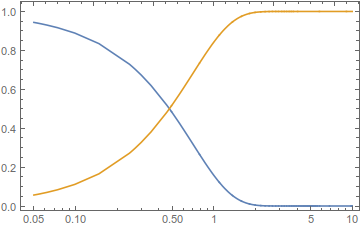
Here is an example:

plot = ParametricPlot[{{x, Erfc[x]}, {x, Erf[x]}}, {x, .05, 10}, 
  PlotRange -> All]

Mathematica graphics

Any plotting options (except for PlotRange) should be given to plotToLogLinearPlot since it effectively redraws the plot from scratch

plotToLogLinearPlot[plot, Frame -> True]

Mathematica graphics

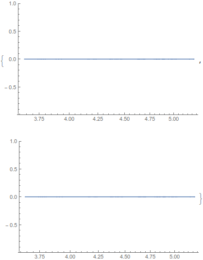
On the code posted in the OP, the log scale is hardly evident since the x-values range from 3.6 to 5.2,

eqnA := {a''[x] + a[x] == b*Sin[a[x]]};
condA := {a[0] == a'[0] == 1};
stopCond := {WhenEvent[Evaluate[Re[a[x]] <= 0], xMax = x;
   "StopIntegration"]}
system := Join[eqnA, condA, stopCond];
sol = ParametricNDSolveValue[system, a, {x, 0, ∞}, {b}];
plot1 = ParametricPlot[(Flatten@
     Last@Transpose[(sol[b])[{"Grid", "ValuesOnGrid"}]]), {b, .8, 2}, 
   PlotRange -> {Automatic, {-1, 1}}];

plot2 = ParametricPlot[(Flatten@
     Last@Transpose[(sol[b])[{"Grid", "ValuesOnGrid"}]]), {b, .8, 2}, 
   PlotRange -> {Automatic, {-1, 1}}];
plotToLogLinearPlot[#, AxesOrigin -> {Automatic, -1}, 
   AspectRatio -> 1/GoldenRatio, PlotRange -> {-1, 1}, 
   ImageSize -> 400] & /@ {plot1, plot2}

Mathematica graphics

$\endgroup$
1
  • $\begingroup$ @ JasonB, your solution is very useful. However, I noted that LogLinearPlot or ListLogLinearPlot effectively generates a curve in which the function is plotted against a logarithm to base $e$. So, could give some suggestion on how to use your method to plot a function with x-axis scaled as a log to base $10$? Thanks! $\endgroup$
    – lxy
    Commented Oct 14, 2016 at 5:26
14
$\begingroup$

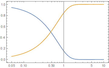
You can use ScalingFunctions. It appears in red but works.

 ParametricPlot[{{x, Erfc[x]}, {x, Erf[x]}}, {x, .05, 10}, 
 PlotRange -> All, ScalingFunctions -> {"Log", Identity}, 
 Frame -> True, AspectRatio -> 0.6]

enter image description here

$\endgroup$
1
  • $\begingroup$ "It appears in red but works"!! I didn't know that was possible. This has broad applicability beyond this problem $\endgroup$ Commented Nov 9, 2023 at 5:15

Your Answer

By clicking “Post Your Answer”, you agree to our terms of service and acknowledge you have read our privacy policy.

Not the answer you're looking for? Browse other questions tagged or ask your own question.