Plotting with Logarithmic Scale

Question

Perhaps this is trivial but I would like to plot the following function:

\begin{equation} p(t)=e^{\left( -\frac{d}{1-c}\right)\left[ W_0\left[B(1+x/r)^{1/d}\right]-W_0[B] \right]} \end{equation} where $W_k$ is the Lambert-W function for the $k=0$ branch and \begin{equation} B=\frac{(1-c)r}{1-(1-c)r}e^{\frac{(1-c)r}{1-(1-c)r}} \end{equation} by the same way they are done in the attached picture below. I am not really sure how to make a $(\log p(x),x)$ plot, but I guess that if I could do one, the $(-\log p(x),x)$ plot would be by ploting $p^{-1}(x)$?

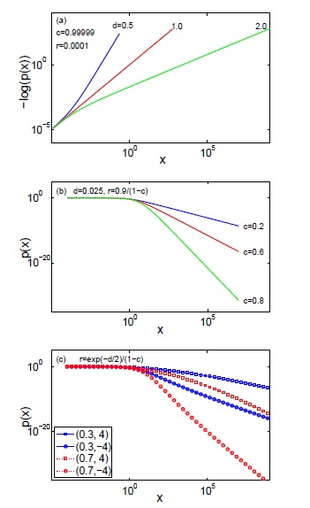
My (poor) attempt so far is the following:

c = 0.99999
r = 0.0001
  B = ((1 - c) r)/(1 - (1 - c) r) Exp[((1 - c) r)/(1 - (1 - c) r)]
   p = Table[ Exp[(-1/(1 - c)) (ProductLog[0, B*(1 + x/r)^(1/1)] - 
   ProductLog[0, B])], {d, 0.5, 2, 0.1}];
   LogPlot[Evaluate[p^-1, {x, 0, 10}], PlotRange -> {10^-1, 10^2}]

But even for the first one I am not able to get them correct.

I would really appreciate your help. Thank you.

Answer 1

Try something like this to define p as a function:

Clear[p]
p[x_, c_, d_, r_] := Module[{B},
  B = ((1 - c) r)/(1 - (1 - c) r) Exp[(1 - c) r/(1 - (1 - c) r)];
  Exp[-d/(1 - c) (ProductLog[0, B*(1 + x/r)^(1/d)] - ProductLog[0, B])]
]

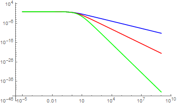
Then something like this to plot multiple instances as a function of different parameter choices:

LogLogPlot[
  {
    p[x, 0.2, 0.025, 0.9/(1 - 0.2)],
    p[x, 0.6, 0.025, 0.9/(1 - 0.6)],
    p[x, 0.8, 0.025, 0.9/(1 - 0.8)]
  },
  {x, 10^-5, 10^9}, PlotRange -> All,
  PlotStyle -> {Blue, Red, Green}
]

Note, however, that I am not sure that your function definition correctly reproduces the values I can infer from the plots you showed. I am also worried about possible issues with numerical precision in your calculations involving very large / very small numbers.

---

Here is a similar idea for the first plot:

LogLogPlot[
  {
    -Log[p[x, 0.99999, 0.5, 1*^-4]],
    -Log[p[x, 0.99999, 1, 1*^-4]],
    -Log[p[x, 0.99999, 2, 1*^-4]]
  },
  {x, 10^-5, 10^9}, PlotRange -> {5*^-6, 1*^4},
  PlotStyle -> {Blue, Red, Green},
  Frame -> True, Axes -> False,
  PlotRangePadding -> {None, {Scaled[0.05], Scaled[0.15]}},
  Epilog -> {
    Inset[
      Style["c=0.99999\nr=0.0001", Black],
      ImageScaled[{0.18, 0.8}], Alignment -> Left
    ],
    Inset[Style["d=0.5", Black], ImageScaled[{0.43, 0.9}]],
    Inset[Style["d=1.0", Black], ImageScaled[{0.66, 0.9}]],
    Inset[Style["d=2.0", Black], ImageScaled[{0.93, 0.8}]]
  }
]