10
$\begingroup$

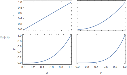
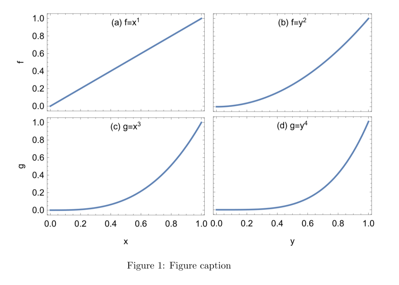
I am writing a document that involves a table of plots, of an array of quantities ($f$ and $g$, say) against an array of variables ($x$ and $y$, say), and which I would like to present in the following form:

I have produced this minimal working example via the following Mathematica code,

fraction = 0.54;
var[1] = "x"; var[2] = "y"; var[3] = "x"; var[4] = "y";
fun[1] = "f"; fun[2] = "f"; fun[3] = "g"; fun[4] = "g";
Grid[Partition[#, 2]] &@
  Table[
   figure[n] = Plot[
     x^n
     , {x, 0, 1}
     , ImageSize -> If[n == 1 || n == 3, fraction 370, (1 - fraction) 370]
     , Frame -> True
     , FrameLabel -> {var[n], fun[n]}
     ,,Epilog->{Inset[Text[Evaluate["("<>{"a","b","c","d"}[[n]]<>") "<>
            fun[n]<>"=\!\(\*SuperscriptBox[\("<>var[n]<>"\), \("<>ToString[n]<>"\)]\)"]],
            Scaled[{0.5,0.97}],Scaled[{0.5,1}]]}
     , ImagePadding -> {{
        If[n == 1 || n == 3, Scaled[0.08], Scaled[0.007]]
        , Scaled[0.01]}, {
        If[n == 3 || n == 4, Scaled[0.08], Scaled[0.007]]
        , Scaled[0.01]}}
     ]
   , {n, 1, 4}];
Table[Export["figure" <> ToString[n] <> ".pdf", figure[n]], {n, 1, 4}]

which then feeds into a simple LaTeX document

\documentclass{article}
\usepackage{graphicx}
\begin{document}
\begin{figure}[h]
\centering
\setlength{\tabcolsep}{0.3mm}
\begin{tabular}{cc}
  \includegraphics[scale=1]{figure1.pdf}&
  \includegraphics[scale=1]{figure2.pdf}\\[-2mm]
  \includegraphics[scale=1]{figure3.pdf}&
  \includegraphics[scale=1]{figure4.pdf}
\end{tabular}
\caption{Figure caption}
\end{figure}
\end{document}

In particular, I want the plots to share scales: I only want to have tick marks and axis labels on the global left and global bottom of the table, because space is at a premium and I want to devote as much space as possible to the plots themselves. This is the reason for the differential use of ImagePadding depending on where in the table each plot sits.

Moreover, I am wedded to the use of scale=1 on the LaTeX figure calls, because I have multiple MaTeX calls on the axis, plot, and tick labels, as well as several other places in the plots, and I want to retain consistency of sizing over all of them. Thus, I want the Exported plots to be produced at the size at which they will be inserted into the LaTeX-produced pdf.

This is a bit problematic, though, because I also want the plot ranges themselves to match up, as exactly as possible, so that the table will be seamless and easier to read. In the code above, this was done by fixing (by hand, and through trial and error) the value of the fraction of the global width that each plot occupies. This mostly works, but it is error-prone and it breaks if there is any sizeable change to the plots, and particularly to the image padding.

This brings me to my question: Is there a way to automate this process? That is, is there a way that I can fix the absolute size, in printer's points, at which the formal PlotRange will be produced within the exported image?

$\endgroup$
3
  • $\begingroup$ Why do you generate 4 pdf files and arrange them in latex? It would be much easier generate the grid layout in Mathematica and export one file. My preferred way for this task is using the package SciDraw. $\endgroup$
    – Felix
    Commented May 7, 2017 at 15:58
  • $\begingroup$ @Felix I find SciDraw to impose a prohibitively high overhead compared to its returns. Arranging things inside Mathematica is an option, but GraphicsGrid is notoriously bad at managing spacings between its constituents, and Grid does not return a Graphics object, which can mess up the export step (particularly if e.g. some plots later need to be exported to png or eps to meet journal requirements). Either way, I think that the specific plot-range-size control I'm asking for is worthwhile on its own. $\endgroup$ Commented May 7, 2017 at 16:05
  • 1
    $\begingroup$ This answer might help $\endgroup$
    – MMA13
    Commented Feb 20, 2019 at 7:03

2 Answers 2

14
+50
$\begingroup$

I don't know if the following addresses all of your issues, but there are 2 things I would try:

  1. ImageSize -> Automatic -> size

This option sets the plot range of the plot to have the ImageSize size.

  1. Charting`ScaledFrameTicks[{Identity, Identity}]

This ticks specification draws tick marks, but no labels.

Using the above, you shouldn't have to worry about tweaking the ImageSize and ImagePadding options. For example:

Grid[{
    {
    Plot[x, {x,0,1}, Frame->True, ImageSize->Automatic->{170,170/GoldenRatio},
        FrameTicks->{{True,True},{Charting`ScaledFrameTicks[{Identity,Identity}],True}},
        FrameLabel->{{f,None}, {None, None}}
    ],
    Plot[y^2, {y,0,1}, Frame->True, ImageSize->Automatic->{170,170/GoldenRatio},
        FrameTicks->{{Charting`ScaledFrameTicks[{Identity,Identity}],True},{Charting`ScaledFrameTicks[{Identity,Identity}],True}}
    ]
    },
    {
    Plot[x^3, {x,0,1}, Frame->True, ImageSize->Automatic->{170,170/GoldenRatio},
        FrameTicks->{{True,True},{Automatic,True}},
        FrameLabel->{{g,None},{x,None}}
    ],
    Plot[y^4, {y,0,1}, Frame->True, ImageSize->Automatic->{170,170/GoldenRatio},
        FrameTicks->{{Charting`ScaledFrameTicks[{Identity,Identity}],True},{Automatic,True}},
        FrameLabel->{{None,None},{y,None}}
    ]
    }
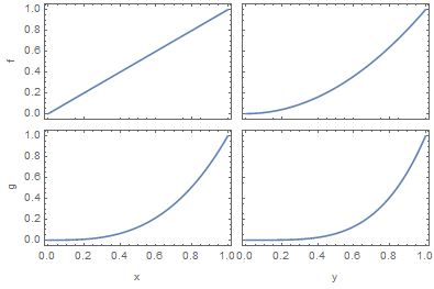
}]

enter image description here

$\endgroup$
2
  • $\begingroup$ That first trick is golden - have you got a good place where it's documented? I don't think it's in the standard docs (which is a worry in terms of stability vs updates changing its behaviour). I'll wait a bit before accepting in case something even better turns up, and I need to test it in my real-world application, but this gets very very close. $\endgroup$ Commented May 7, 2017 at 17:17
  • $\begingroup$ Sadly ImageSize -> Automatic -> size is ignored by Inset: Graphics[{Inset[Plot[x^3,{x,0,1},Frame->True,ImageSize->Automatic->{170,170/GoldenRatio},FrameLabel->{{y,y},{x,x}}],{0,0},Scaled[{0,0}],Automatic]}]. Is it possible to make it working with Inset? $\endgroup$ Commented May 8, 2017 at 7:06
5
$\begingroup$

Here is an approach based on well-documented Inset[gr, pos, opos, Automatic] functionality.

It is important to use Scaled specification for opos. Benefits:

  1. Using Scaled specification for opos we position inset relative to the corners of its plotting range, not relative to the image corners.

  2. We can safely add any ImagePadding to gr without altering its position.

Having this in mind, we first choose a convenient constant ImagePadding for all insets with which we won't care anymore about possibility of cropping in insets themselves:

iP = 100;

Desired size of the plotting range:

{iPRW, iPRH} = {170, 170/GoldenRatio};

Since ImagePadding is included in ImageSize, the final ImageSize for insets is calculated as sum of the size of the plotting range plus doubled ImagePadding:

iS = {iPRW, iPRH} + 2 iP;

We have to choose horizontal and vertical spacings between plots in the final grid:

{hSpacing, vSpacing} = {10, 10};

ImagePadding for the whole figure is the only parameter which we tune by hand (although there is a way to obtain it automatically):

iPGrid = {{40, 5}, {40, 3}};

Having it we can calculate the size of the final figure:

iSGrid = 2*{iPRW, iPRH} + {hSpacing, vSpacing} + Plus @@@ iPGrid;

Now the plotting part.

Abbreviations (a fix for this bug is included in t):

opts = Sequence[Frame -> True, ImageSize -> iS, ImagePadding -> iP];
t = Charting`ScaledFrameTicks[{Identity, Identity}][##][[;; , ;; 3]] &;

Our plots (taking setup of Carl Woll):

plots = With[{opts = opts}, {
    {Plot[x, {x, 0, 1}, opts, FrameTicks -> {{True, True}, {t, True}}, 
      FrameLabel -> {{"f", None}, {None, None}}],
     Plot[y^2, {y, 0, 1}, opts, FrameTicks -> {{t, True}, {t, True}}]},
    {Plot[x^3, {x, 0, 1}, opts, FrameTicks -> {{True, True}, {True, True}}, 
      FrameLabel -> {{"g", None}, {"x", None}}],
     Plot[y^4, {y, 0, 1}, opts, FrameTicks -> {{t, True}, {True, True}}, 
      FrameLabel -> {{None, None}, {"y", None}}]}}];

Now we assemble everything into the final figure. It is important to set AspectRatio -> Full in order to avoid cropping:

grid = Graphics[{
   Inset[plots[[2, 1]], {0, 0}, Scaled[{0, 0}], Automatic],
   Inset[plots[[2, 2]], Offset[{iPRW + hSpacing, 0}, {0, 0}], Scaled[{0, 0}], Automatic],
   Inset[plots[[1, 1]], Offset[{0, iPRH + vSpacing}, {0, 0}], Scaled[{0, 0}], Automatic],
   Inset[plots[[1, 2]], Offset[{iPRW + hSpacing, iPRH + vSpacing}, {0, 0}], 
    Scaled[{0, 0}], Automatic]},
  ImageSize -> iSGrid, AspectRatio -> Full, PlotRange -> {{0, 1}, {0, 1}}, 
  ImagePadding -> iPGrid]

output

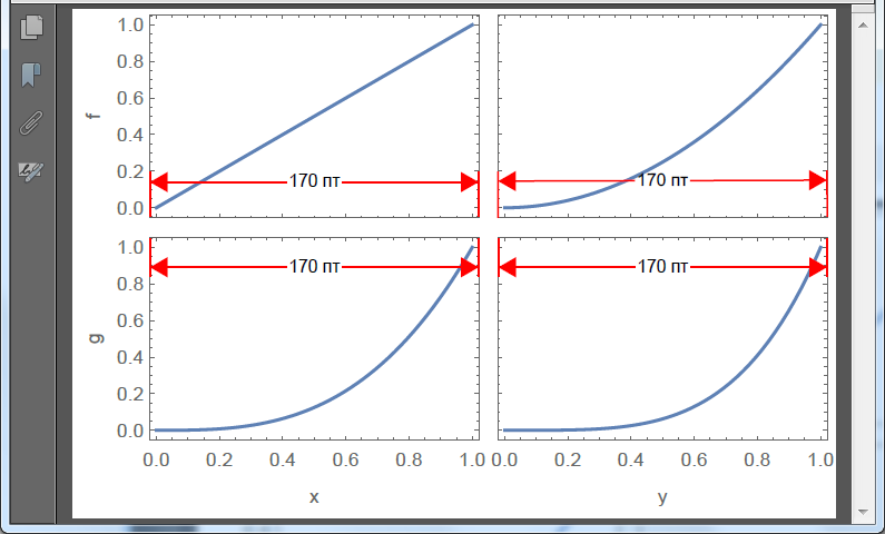
Let us check the sizes of the plotting areas using Adobe Acrobat's "Measurement tool":

Export["grid.pdf", grid] // SystemOpen

screesnhot

$\endgroup$

Your Answer

By clicking “Post Your Answer”, you agree to our terms of service and acknowledge you have read our privacy policy.

Not the answer you're looking for? Browse other questions tagged or ask your own question.