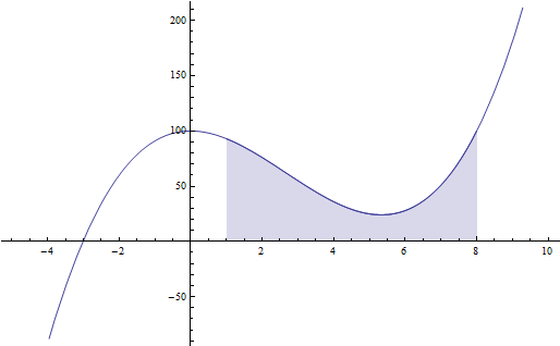
I would like to visualize what it graphically means to integrate between two boundary values. Therefore I'd like to make a Filling between these two values. Is there a way to get this done?
-
1$\begingroup$ Something like this (source code is free there) ?demonstrations.wolfram.com/IntegrationIsASum $\endgroup$– Vitaliy KaurovCommented Aug 21, 2012 at 8:03
6 Answers
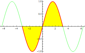
An alternative is to use Piecewise as follows
Plot[{Sin[x], Piecewise[{{Sin[x], -Pi <= x <= Pi}}, _]}, {x, -2 Pi, 2 Pi},
  Filling -> {2 -> {Axis, Yellow}}, PlotStyle -> {Green, Directive[Red, Thick]}]
which gives
Or
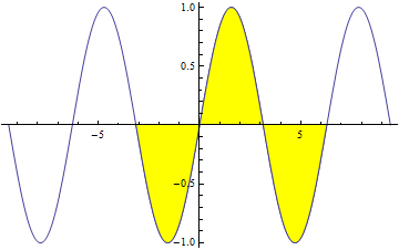
Use Show to superimpose two variants (the second one with your choice of the variable bounds -- -Pi and 2Pi in the example below) of the plot:
Show[Plot[Sin[x], {x, -3 Pi, 3 Pi}],
     Plot[Sin[x], {x, - Pi, 2 Pi},
         Filling -> Axis, FillingStyle -> Yellow]]
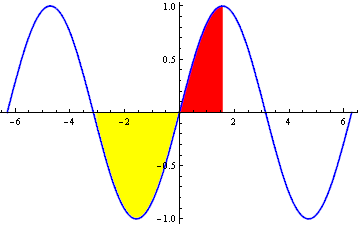
Update: Yet another method using ColorFunction with ColorFunctionScaling->False, Mesh and MeshShading,
Plot[Sin[x], {x, -2 Pi, 2 π},
   Mesh -> {{0}},
   MeshShading -> {Directive@{Thick, Blue}}, Filling -> Axis,
   ColorFunction -> (If[-Pi <= #1 <= Pi/2, If[#2 > 0, Red, Yellow], White] &),
   ColorFunctionScaling -> False]
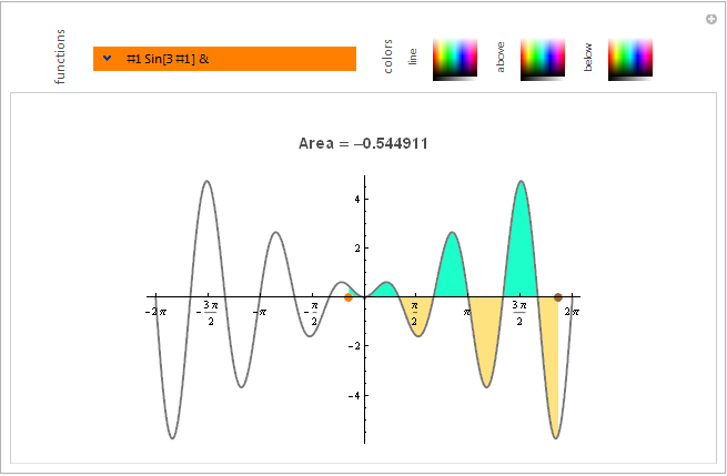
Update 2: All inside Manipulate:
First, a cool combo control from somewhere in the docs:
 popupField[Dynamic[var_], list_List] :=
   Grid[{{PopupMenu[Dynamic[var], list, 0,
          Opener[False, Appearance -> Medium]],
          InputField[Dynamic[var], Appearance -> "Frameless"]}},
  Frame -> All, FrameStyle -> Orange,
  Background -> {{Orange, Orange}}]
and, then,
Manipulate[Column[{ Dynamic@Show[ Plot[func[x], {x, -2 Pi, 2 π},
  Ticks -> {Range[-2 Pi, 2 Pi, Pi/2], Automatic},
  Mesh -> {{0}}, MeshShading -> {Directive@{Thick, color0}},
  Filling -> Axis,
  ColorFunction -> (If[lb <= #1 <= ub, If[#2 > 0, color1, color2], White] &),
  ColorFunctionScaling -> False, ImageSize -> {600, 300}],
  Graphics[{Gray, Line[{{-2 Pi, 0}, {2 Pi, 0}}],
   Orange, PointSize[.02], Dynamic[(Point[{lb = Min[First[pt1], First[pt2]], 0}])],
   Brown, PointSize[.02],  Dynamic[(Point[{ub = Max[First[pt1], First[pt2]], 0}])]},
  PlotRange -> 1.], PlotLabel -> Style[ "\nArea = " <>
    ToString[Quiet@NIntegrate[func[t], {t, lb, ub}]] <> "\n",
   "Subsection", GrayLevel[.3]]]},  Center],
 Row[{Spacer[30], Rotate[Style["functions", GrayLevel[.3], 12], 90 Degree],
  Spacer[5],Control@{{func, Sin, ""},  popupField[#, {Sin, Cos, Sec, Cosh, ArcSinh}] &}
  Spacer[15], Rotate[Style["colors", GrayLevel[.3], 12], 90 Degree],
  Spacer[5],  Rotate[Style["line", GrayLevel[.3], 10], 90 Degree],
  Control@{{color0, Blue, ""}, ColorSlider[#, AppearanceElements -> "Spectrum",
           ImageSize -> {40, 40}, AutoAction -> True] &},
 Spacer[5], Rotate[Style["above", GrayLevel[.3], 10], 90 Degree],
 Control@{{color1, Green, ""}, ColorSlider[#, AppearanceElements -> "Spectrum",
          ImageSize -> {40, 40}, AutoAction -> True] &},
 Spacer[5], Rotate[Style["below", GrayLevel[.3], 10], 90 Degree],
 Control@{{color2, Green, ""}, ColorSlider[#, AppearanceElements -> "Spectrum",
           ImageSize -> {40, 40}, AutoAction -> True] &}},Spacer[0]],
 {{lb, -Pi}, ControlType -> None},
 {{ub, 3 Pi/2}, ControlType -> None},
 {{pt1, {-Pi, 0}}, Locator, Appearance -> None},
 {{pt2, {3 Pi/2, 0}}, Locator, Appearance -> None},
 Alignment -> Center, ControlPlacement -> Top, AppearanceElements -> Automatic]
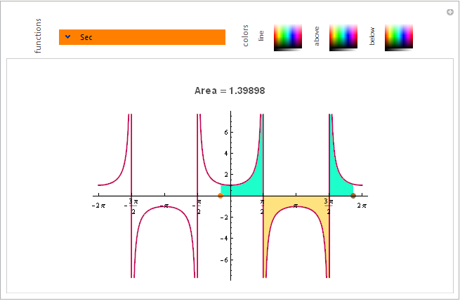
Enter your own pure function:
-
$\begingroup$ Thank you for your answer. I liked the second code snippet of yours with the Show command, the best. One thing though, the filling is better done with Filling->0 instead of Filling->Axis $\endgroup$ Commented Jan 17, 2017 at 18:41
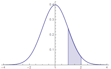
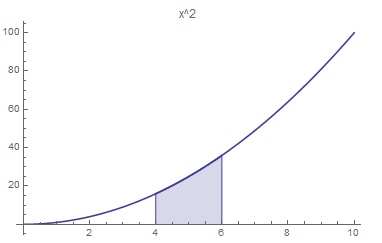
I made an answer by J.M. and Murta into a function:
IntegralPlot[f_, {x_, L_, U_}, {l_, u_}, opts : OptionsPattern[]] :=
 Module[{col = ColorData[1, 1]},
  Plot[{ConditionalExpression[f, x > l && x < u], f},
   {x, L, U},
   Prolog -> {{col, Line[{{l, 0}, {l, f /. {x -> l}}}]}, {col,
      Line[{{u, 0}, {u, f /. {x -> u}}}]}},
   Filling -> {1 -> Axis},
   PlotStyle -> col,
   opts]]

IntegralPlot[PDF[NormalDistribution[0, 1]][x], {x, -4, 4}, {1, 2}]
IntegralPlot[x^2, {x, 0, 10}, {4, 6}, PlotLabel -> "x^2"]
-
1$\begingroup$ Nice idea to capture the functionality within a function. $\endgroup$ Commented Nov 23, 2014 at 15:00
With axis-constrained locators:
DynamicModule[{pts = {{0, 0}, {Pi, 0}}},
 LocatorPane[Dynamic[pts, (pts[[1]] = {#[[1, 1]], 0}; pts[[2]] = {#[[2, 1]], 0}) &],
 Dynamic[
   Framed@Show@
          {Plot[Sin@x, {x, 0, 2 Pi}],
           Plot[Sin@x, {x, pts[[1, 1]], pts[[2, 1]]}, Filling -> Axis]
          }
   ]]]
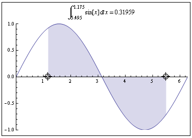
Edit
This is the full code, with the label:
DynamicModule[{pts = {{0, 0}, {Pi, 0}}},
 LocatorPane[Dynamic[pts, (pts[[1]] = {#[[1, 1]], 0}; pts[[2]] = {#[[2, 1]], 0}) &],
 Dynamic[
   Framed@Show@
          {Plot[Sin@x, {x, 0, 2 Pi},
            PlotLabel -> ToString@StandardForm[Integrate[sin[x],
                         {x, pts[[1, 1]], pts[[2, 1]]}]] <> " = " <>
                         ToString[Integrate[Sin@x, {x, pts[[1, 1]], pts[[2, 1]]}]]],

           Plot[Sin@x, {x, pts[[1, 1]], pts[[2, 1]]}, Filling -> Axis]
          }
   ]]]
Area will be red or blue depending whether $b > a$ or not.
Manipulate[
  Plot[{f[x], UnitStep[Sign[b - a] (x - a)] UnitStep[Sign[b - a] (b - x)] f[x]},
    {x, -7, 7}, PlotStyle -> {Thick, Thickness[0]}, Filling -> {2 -> 0},
  FillingStyle -> Directive[Opacity[.5], If[b - a > 0, Red, Blue]],
  PlotLabel -> "AREA = " <> ToString[NIntegrate[f[x], {x, a, b}]]], {{b, 4}, -7, 7},
   {{a, -1}, -7, 7}, {f, {Sin, Cos, Tanh, Sech}}]
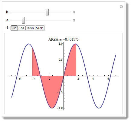
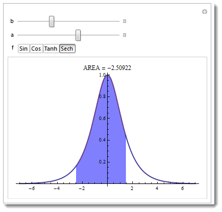
Also take a look at source code at the Wolfram Demonstration Project.
Copying the second code snippet of user kglr's answer I changed the command Filling->Axis into Filling->0.
(*start*)
integrationLimit1 = 1;
integrationLimit2 = 8;
f[x_] = 100 - 8*x^2 + x^3;
g1 = Plot[f[x], {x, -5, 10}];
g2 = Plot[f[x], {x, integrationLimit1, integrationLimit2},
   Filling -> 0];
Show[g1, g2]
(*end*)
Also, the order of the graphics g1 and g2 in the Show command are important.
Always search the doc when you don't know what to do. In most cases you'll not only find it possible, but find a thorough documentation along with examples. In this case you have this link.
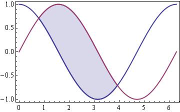
Here is an example:
Show[
 Plot[{Cos[x], Sin[x]}, {x, 0, 2 π}],
 Plot[{Cos[x], Sin[x]}, {x, π/4, 5/4 π},
     PlotRange -> {{0, 2 π}, All} , Filling -> 1 -> {2}]
]
-
$\begingroup$ Thx for the answer, but what I would like to do is to shade just one of these function between two boundary values. $\endgroup$– RMMACommented Aug 21, 2012 at 8:12
-
$\begingroup$ @rainer I simply supplied an example. If you want to fill it in alternatively look through the documentation for Filling. $\endgroup$– jVincentCommented Aug 21, 2012 at 8:40

