77
$\begingroup$

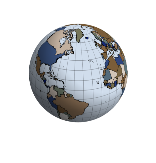
There are many ways to create a 3D Earth that is rotatable (see here, here, related here), but most of them have some drawbacks. These issues mainly stem from either CountryData or the fact that 3D shapes are not easy to handle. How can one efficiently overcome these problems? How to create a 3D rotateable, high-resolution-textured or polyon-based, fast-response, good-looking Earth?

Update:

Specific problem to solve: Given a 3D Earth, how can a 2D plot be layered on the surface such that only those parts of the plot appear that are above continents?

In other words: How to plot a species' distribution over the globe? My present method is quite tedious and is really slow. It involves the creation of a continent-texture map, the rasterization of some random distribution patches (any will suffice, mine is taken from here), some image-processing algorithm to color the intersection of continents and the distribution (as Mathematica lacks proper polygon-intersection tools at the moment), and projecting the result over the sphere. This has various problems apart from slowness (see below the example). Following is a test-creature that was obliterated from the Italian Peninsula.
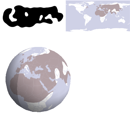
Mathematica graphics

Here I list the methods known to me to create the globe, and their shortcomings:

1. Make a 3D wireframe from polygon data

Extract 2D polygon data for each country & continent from CountryData, convert them to 3D and project coordinates to a sphere. Issues:

  • looks ugly if only "SchematicPolygon"-s are used (too few points)
  • too much computation if "FullPolygon"-s are used (too many points)
  • edge transparency slows down interactive manipulation terribly, though for aesthetics, it is needed sometimes
  • no perfect way to put a sphere under the wireframe to prevent see-through, or to put e.g. a vegetation map texture to go with the vector-country-borders (see next)
  • no easy way to make countries filled polygons, as it either creates artefacts (fill goes out of boundary, unclosed polygons, etc.) or interferes with sphere surface (if present under the wireframe), as polygons are not bent according to the curvature of the globe.

Example:

mapData = CountryData[#, "SchematicPolygon"] & /@ 
   Flatten[CountryData /@ CountryData["Continents"]];
SC[{lat_, lon_}] := {Cos[lon \[Degree]] Cos[lat \[Degree]], 
   Sin[lon \[Degree]] Cos[lat \[Degree]], Sin[lat \[Degree]]};
mapDataSphere = 
  Flatten@(mapData /. n : {_Real, _Real} :> SC@Reverse@n);
Graphics3D[{Hue[.58, .1, 1], FaceForm@White, 
  EdgeForm@{[email protected], [email protected]}, mapDataSphere}, 
 ImageSize -> 300, Boxed -> False]
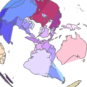
Mathematica graphics

2. Make a texture bitmap and project it onto a sphere

Create a high-resolution 2D map of the world, and apply it to e.g. SphericalPlot3D. It produces a globe that can be rotated quite easily, though it has other issues:

  • By using textures, one looses all the advantages of vector graphics. For example any change to the surface map involves image processing (i.e. layering a species' distribution over the continents), which is usually slow, especially for textures of high resolution.
  • The resolution of the texture map does not seem to be used for its full extent, as the applied texture looks less crisp than the original 2D map.
  • SphericalPlot3D produces artefacts (holes in the surface, weird shadow at boundary)
  • If the texture map is not rasterized before, it produces artefacts (see lines across North America)

Examples:

mapData = 
  CountryData[#, "FullPolygon"] & /@ 
   Flatten[CountryData /@ CountryData["Continents"]];    
map = Graphics[{White, EdgeForm@{Gray, AbsoluteThickness@0}, mapData},
        ImageSize -> 2000, PlotRangePadding -> 0, 
       PlotRange -> {{-180, 180}, {-90, 90}}, 
       Background -> Hue[.58, .1, 1]];
SphericalPlot3D[1, {u, 0, Pi}, {v, 0, 2 Pi}, 
     TextureCoordinateFunction -> ({#5 + .5, 1 - #4} &), 
     PlotStyle -> Texture@map, SphericalRegion -> True, Axes -> False, 
     Boxed -> False, Lighting -> "Neutral", Mesh -> False, 
     PlotRangePadding -> 0, RotationAction -> "Clip", ImageSize -> 300]
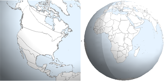
Mathematica graphics

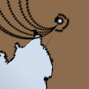
Various artefacts in Mark's answer, when zoomed on to the South Pole:
Mathematica graphics

Note polygon spiral-lines (polygon issue, can be cured by rasterization); low resolution (can be increased, but not to a level when zooming on like this does not reveal pixels); the alignment issue at the surface boundary (thin blue line pointing to the pole) due to 3D plotting; and the blue point right at the pole (projection issue).

3. Simulate 3D with high-resolution bitmap in 2D

This is a hypothetic way I haven't tried. First, create a large bitmap of the world. Tile the space periodically with it, and use an orthographic projection to simulate a 3D sphere-like lens effect whenever the map is dragged by the mouse. By this way 3D can be simulated in 2D. Could be faster than the texture mapped sphere.

Texture map issues

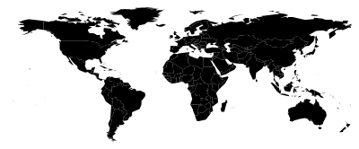
Why is it that many geographic features are not shown consistently by CountryData? I would assume this returns a full world map, but I guess since Antarctica is not a sovereign country, it is omitted:

Graphics[CountryData[#, "SchematicPolygon"] & /@ CountryData[All], ImageSize -> 400]
Mathematica graphics

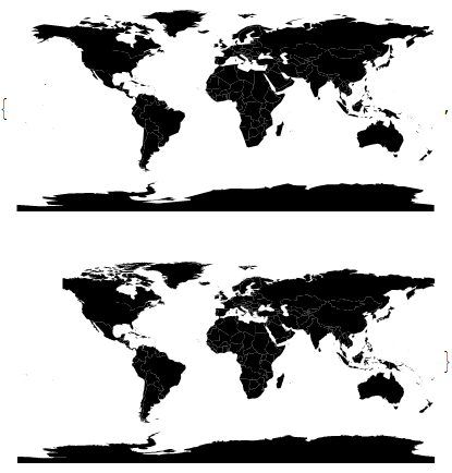
But I cannot explain the missing features of the second plot below (e.g. Alaska). How come that the "Polygon" specification, that is supposed to be more detailed than "SchematicPolygon", is actually missing features the other has?

{
Graphics[CountryData[#, "SchematicPolygon"] & /@ CountryData["Continents"], ImageSize -> 400],
Graphics[CountryData[#, "Polygon"] & /@ CountryData["Continents"], ImageSize -> 400]
}
Mathematica graphics

$\endgroup$
13
  • $\begingroup$ I've extended the scope of the question as it seems to generate more useful answers. If you think the new stuff should rather go to a completely new post, please say so. $\endgroup$ Commented Mar 29, 2012 at 3:01
  • $\begingroup$ To avoid the strange spirals I used: Texture[Rasterize[pic, ImageSize -> 1500]] instead of Show in Mark's code. $\endgroup$
    – FJRA
    Commented Mar 29, 2012 at 16:10
  • $\begingroup$ Can you make the data describing your region available? $\endgroup$ Commented Apr 24, 2012 at 1:18
  • 3
    $\begingroup$ While I'm a huge proponent of OPs editing their question to update with more info, here, the question went from 1) "What's the logic behind CountryData" to 2) "How to make a 3D globe" to now 3) "Plot geographic data over a 3D globe" over the course of a month! I think this is excessive— questions should be updated with info, not changed in scope! It makes Fx's and FJRA's answers look completely out of place. It's also on the verge of being bumped to CW, for those who care. I think that this should've been 3 separate questions or one well thought out question. It's too late to do anything now $\endgroup$
    – rm -rf
    Commented Apr 24, 2012 at 1:52
  • $\begingroup$ @R.M Yes, I agree with you, though on the other hand, I did feel that they are heavily intertwined issues: I've tried many things, and realized that if I change e.g. the method of graphics-intersection then I have to change the method of projection as well. And to be honest, when I posted this thing weeks ago I had the intention to post exactly the question I asked yesterday. But since I was way behind my idea, I had to do my research in the meantime. I know that it is now a complex issue, that's why I've tried to soften the blow with the bounty. $\endgroup$ Commented Apr 24, 2012 at 9:54

4 Answers 4

66
+250
$\begingroup$

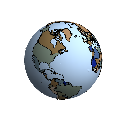
This answer was originally posted in 2012 and based on version 8 of Mathematica. Since then, a number of changes have made it possible to generate the globe in much less code. Specifically:

  • CountryData[_,"SchematicPolygon"] now returns polygons of sufficient resolution to make a nice globe. Thus, we don't need to apply polyline simplification to FullPolygons.
  • Triangulation is now built in.

Thus, we can now generate the globe as follows:

countryComplex[country_] := Module[
  {boundaryPts, mesh, g, triPts, tris, pts3D, linePts, lines, linePts3D},
  boundaryPts = Map[Reverse, 
        CountryData[country, "SchematicCoordinates"], 
    {2}];
  mesh = TriangulateMesh[Polygon[boundaryPts]];
  g = Show[mesh];
  {triPts, tris} = {g[[1, 1]], g[[1, 2, 2, 1, 1, 1]]};
  pts3D = Map[
        Normalize[First[
            GeoPositionXYZ[GeoPosition[Reverse[#]]]
        ]] &, triPts];
  g = Show[RegionBoundary[mesh]];
  {linePts, lines} = {g[[1, 1]], g[[1, 2, 2, 1, 1, 1]]};
  linePts3D = Map[
        Normalize[First[
            GeoPositionXYZ[GeoPosition[Reverse[#]]]
        ]] &, linePts];
  {GraphicsComplex[pts3D, 
        {EdgeForm[], ColorData["DarkTerrain"][Random[]], Polygon[tris]}, 
        VertexNormals -> pts3D],
   GraphicsComplex[linePts3D, {Thick, Line[lines]}]}
];

SeedRandom[1];
complexes = countryComplex /@ Prepend[CountryData[All], "Antarctica"];
pic = Graphics3D[{{ColorData["Aquamarine"][3], 
  Sphere[{0, 0, 0}, 0.99]}, complexes}, 
  Lighting -> "Neutral", Boxed -> False]

enter image description here


Orginal 2012 Answer

I'm posting this as a second answer, as it's really a completely different approach. It's also been substantially expanded as of April 25, 2012. While this still doesn't specifically address the question of adding a region, it does plot the countries separately. Of course, each country could be viewed as a region in itself.

Our objective is to make a good, genuine 3D globe. We prefer not to use a texturized parametric plot, for then we we'll have distortion at the poles and no access to the graphics primitives making the image.

It's quite easy to project data given as (lat,lng) pairs onto a sphere using GeoPosition and related functions (or even just the standard parametrization of a sphere). However, the SchematicPolygon returned by CountryData are of insufficient resolution to generate a truly nice image while the FullPolygons are so detailed that the resulting 3D object is clunky to interact with. Furthermore, non-convex 3D polygons tend to render poorly in Mathematica with the fill leaking out.

Our solution is two-fold. First, we simplify the FullPolygons to a manageable but still detailed level. Second, we triangulate the resulting polygons before projecting onto the sphere. Note that we use a third party program called triangle for the triangulation. Once installed, however, the procedure can be carried out entirely within Mathematica using the Run command.

Polyline simplification

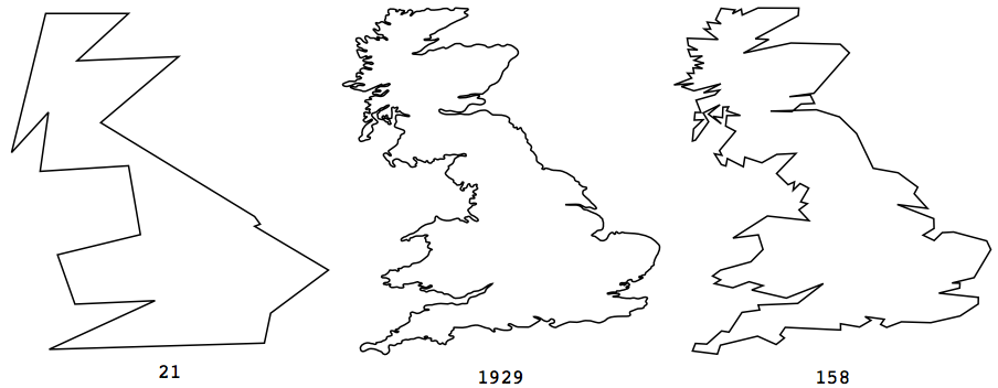
Here are the Schematic and Full Polygons returned by CountryData for Britain, known for it's complicated coastline. Note that the FullPolygon consists of nearly 4000 total points, while the SchematicPolygon has only 26.

pts[0] = Map[Reverse, 
  CountryData["UnitedKingdom", "SchematicCoordinates"], {2}];
pts[1] = Map[Reverse, 
  CountryData["UnitedKingdom", "FullCoordinates"], {2}];
Total /@ Map[Length, {pts[0], pts[1]}, {2}]

{26, 3924}

In order to plot a nice image that is easy to interact with, we've really got to reduce the number of points in the FullPolygon. A standard algorithm for reducing points while maintaining the integrity of the line is the Douglas-Peucker algorithm. Here is an implementation in Mathematica:

dist[q : {x_, y_}, {p1 : {x1_, y1_}, p2 : {x2_, y2_}}] := With[
   {u = (q - p1).(p2 - p1)/(p2 - p1).(p2 - p1)},
   Which[
    u <= 0, Norm[q - p1],
    u >= 1, Norm[q - p2],
    True, Norm[q - (p1 + u (p2 - p1))]
    ]
   ];
testSeg[seg[points_List], tol_] := Module[{dists, max, pos},
    dists = dist[#, {points[[1]], points[[-1]]}] & /@ 
      points[[Range[2, Length[points] - 1]]];
    max = Max[dists];
    If[max > tol,
     pos = Position[dists, max][[1, 1]] + 1;
     {seg[points[[Range[1, pos]]]], 
      seg[points[[Range[pos, Length[points]]]]]},
     seg[points, done]]] /; Length[points] > 2;
testSeg[seg[points_List], tol_] := seg[points, done];
testSeg[seg[points_List, done], tol_] := seg[points, done];
dpSimp[points_, tol_] := 
  Append[First /@ First /@ Flatten[{seg[points]} //. 
       s_seg :> testSeg[s, tol]], Last[points]];

Let's illustrate with the coast of Britain. The second parameter is a tolerance; a smaller tolerance yields a better approximation but uses more points. The implementation doesn't like the first and last points to be the same, hence we use Most. Finally, we can toss out parts that yield just two points after simplification, since they will be very small.

pts[2] = Select[dpSimp[Most[#],0.1]& /@ pts[1], Length[#]>2&];
Total[Length /@ pts[2]]

341

The result has only 341 total points. Let's look at the mainland.

Row[Table[Labeled[Graphics[{EdgeForm[Black],White,
  Polygon[First[pts[i]]]}, ImageSize -> 200],
  Length[First[pts[i]]]],{i,0,2}]]

enter image description here

Our simplified polygon uses only 158 points for mainland Britain to yield an approximation that should look good on a globe.

Triangulation

Triangulation is an extremely important topic in computational geometry and still a topic in current research. Our topic here illustrates it's importance in computer graphics; it is also very important in the numerical solution of PDEs. It is surprisingly hard to do well in full generality. (Consider, for example, that our simplified polygons are not guaranteed to be simple, i.e. they may and probably do self-intersect.) Unfortunately, Mathematica doesn't have a built in triangulation procedure as of V8. Rather than start from scratch, I've written a little interface to the freely available program called triangle: http://www.cs.cmu.edu/~quake/triangle.html

Installing triangle on a unix based system, like Mac OS X, was easy enough for me - though, it does require some facility with C compilation. I don't know about Windows. Once you've got it set up to run from the command line, we can access it easily enough through Mathematica's Run command by reading and writing triangle files. Let's illustrate with the boundary of Britain again.

Triangle represents polygons using poly files. The following code writes a sequence of points to a stream in poly file format.

toPolyFile[strm_, pts : {{_, _} ..}] := Module[{},
   WriteString[strm, ToString[Length[pts]] <> " 2 0 0\n"];
   MapIndexed[
    WriteString[strm, 
      ToString[First[#2]] <> " " <>
       ToString[First[#]] <> " " <>
        ToString[Last[#]] <> "\n"] &, pts];
   WriteString[strm, ToString[Length[pts]] <> " 0\n"];
   Do[WriteString[strm, 
     ToString[i] <> " " <> ToString[Mod[i - 1, Length[pts], 1]] <> 
      " " <> ToString[i] <> "\n"],
    {i, 1, Length[pts]}];
   WriteString[strm, "0"]
   ];

For example, we can write poly files for the british coast approximations as follows.

Do[
  strm = OpenWrite["BritishCoast"<>ToString[i]<>".poly"];
  toPolyFile[strm,First[pts[i]]];
  Close[strm],
{i,0,2}]

We'll triangulate using the following command.

$triangleCmd = "/Users/mmcclure/Documents/triangle/triangle -pq ";

Here's the actual triangulation step.

Do[
  Run[$triangleCmd<>"BritishCoast"<>ToString[i]<>".poly"],
{i,0,2}]

This produces new poly files as well as node and ele files. These can be read back in and translated to GraphicsComplexs.

triangleFilesToComplex[fileName_String, itNumber_:1] := 
  Module[{pts, triangles, edges, data},
   data = Import[fileName <> "." <> ToString[itNumber] <> ".node",  "Table"];
   pts = #[[{2, 3}]] & /@ data[[2 ;; -2]];
   data = Import[fileName <> "." <> ToString[itNumber] <> ".ele", "Table"];
   triangles = Rest /@ data[[2 ;; -2]];
   data = Import[fileName <> "." <> ToString[itNumber] <> ".poly", "Table"];
   edges = #[[{2, 3}]] & /@ data[[3 ;; -3]];
   GraphicsComplex[pts, {
     {White, EdgeForm[{Black,Thin}], Polygon[triangles]},
     {Thick, Black, Line[edges]}}]]

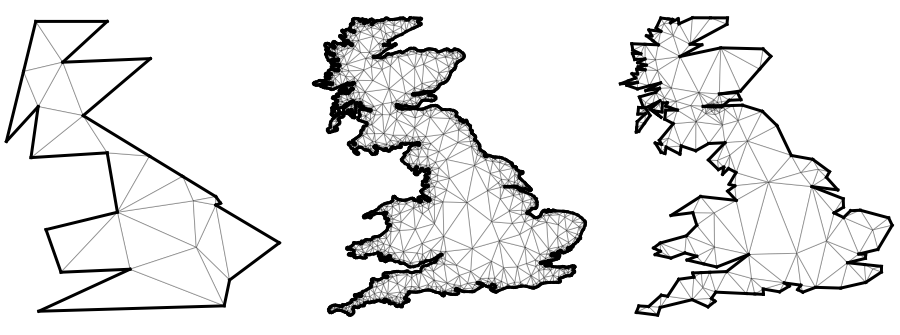
Here's the result.

GraphicsRow[Table[
  Graphics[triangleFilesToComplex["BritishCoast"<>ToString[i]]],
{i,0,2}], ImageSize -> 600]

enter image description here

The Globe

OK, let's put this all together to generate the globe. The procedure will generate a huge number of files, so let's set up a directory in which to store them. (Unix specific)

SetDirectory[NotebookDirectory[]];
If[FileNames["CountryPolys"] === {},
  Run["mkdir CountryPolys"],
  Run["rm CountryPolys/*.poly CountryPolys/*.node CountryPolys/*.ele"]
];

The next command is analogous to the toPolyFile command above, but accepts a country name as a string, generates poly files for all the large enough sub-parts, and triangulates them.

$triangleCmd = "/Users/mmcclure/Documents/triangle/triangle -pq ";
triangulateCountryPoly[country_String] := 
  Module[{multiPoly, strm, fileName, len, fp},
   fp = CountryData[country, "FullCoordinates"];
   multiPoly = Select[dpSimp[Most[#], 0.2] & /@ fp, Length[#] > 2 &];
   len = Length[multiPoly];
   Do[
    fileName = "CountryPolys/" <> country <> ToString[i] <> ".poly";
    strm = OpenWrite[fileName];
    toPolyFile[strm, multiPoly[[i]]];
    Close[strm];
    Run[$triangleCmd <> fileName], 
    {i, 1, len}];
   ];

Next, we need a command to read in a triangulated country (consisting of potentially many polygons) and store the result in a GraphicsComplex.

toComplex3D[country_String] := 
  Module[{len, pts, pts3D, ptCnts, triangles, edges, data},
   Catch[
    len = 
     Length[FileNames[
       "CountryPolys/" <> country ~~ NumberString ~~ ".1.poly"]];
    pts = Table[
      data = 
       Check[Import[
         "CountryPolys/" <> country <> ToString[i] <> ".1.node", 
         "Table"], Throw[country]];
      #[[{2, 3}]] & /@ data[[2 ;; -2]], {i, 1, len}];
    ptCnts = Prepend[Accumulate[Length /@ pts], 0];
    pts = Flatten[pts, 1];
    triangles = Flatten[Table[
       data = 
        Check[Import[
          "CountryPolys/" <> country <> ToString[i] <> ".1.ele", 
          "Table"], Throw[country]];
       ptCnts[[i]] + Rest /@ data[[2 ;; -2]], {i, 1, len}], 1];
    edges = Flatten[Table[
       data = 
        Check[Import[
          "CountryPolys/" <> country <> ToString[i] <> ".1.poly", 
          "Table"], Throw[country]];
       ptCnts[[i]] + (#[[{2, 3}]] & /@ data[[3 ;; -3]]), {i, 1, len}],
       1];
    pts3D = 
     Map[Normalize[First[GeoPositionXYZ[GeoPosition[Reverse[#]]]]] &, 
      pts];
    GraphicsComplex[pts3D,
     {{EdgeForm[], ColorData["DarkTerrain"][Random[]], 
       Polygon[triangles]},
      {Line[edges]}}, VertexNormals -> pts3D]
    ]
];

OK, let's do it.

countries = Prepend[CountryData[All], "Antarctica"];
triangulateCountryPoly /@ countries; // AbsoluteTiming

{77.350341, Null}

SeedRandom[1];
complexes = toComplex3D /@ countries; // AbsoluteTiming

{94.657840, Null}

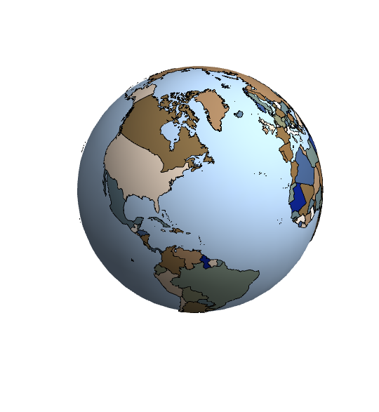
globe = Graphics3D[{
  {ColorData["Aquamarine"][3], Sphere[{0, 0, 0}, 0.99]}, complexes},
  Lighting -> "Neutral", Boxed -> False]

enter image description here

$\endgroup$
9
  • $\begingroup$ This is a promising approach! Could you please tell something about the performance of the FullPolygon-ed globe, whether it is fast to rotate, or does it lag? $\endgroup$ Commented Mar 30, 2012 at 17:43
  • $\begingroup$ @Istvan The FullPolygon version is rotatable, but barely. It's jerky and has crashed my computer twice in four tries. The compressed Graphics3D object is 32Mb. If you really need something finer than SchematicPolygons, then you could possibly take the FullPolygons and run them through a point reduction algorithm. The problem there is that it can be difficult to preserve the topological properties, i.e. the polygon may end up intersecting itself. $\endgroup$ Commented Mar 30, 2012 at 19:13
  • 1
    $\begingroup$ @Mr.Wizard I've not tried that package. I'd be a bit surprised though if it does work. The obvious polygon to try it on is First[CountryData["Norway", "Coordinates"]]. $\endgroup$ Commented Apr 9, 2012 at 21:03
  • 2
    $\begingroup$ @MarkMcClure I like the polygon coarsening algorithm. How would you make sure that neighbouring countries still match after the process? $\endgroup$
    – Heike
    Commented Apr 26, 2012 at 15:49
  • 1
    $\begingroup$ This is a really detailed and heavyweight solution, thank you for all the effort you put into it! One solution for @Heike's concern would be to triangulate full continents, and later add simplified lines for inland borders. This way of course one cannot color countries independently but if that is not important (like for me) the outcome might be even smaller in filesize than your result. Anyway, it definitely worths the bounty, thanks again! $\endgroup$ Commented Apr 29, 2012 at 23:32
34
$\begingroup$

This is not a direct response to the question but rather a response to Istvan's comment to FJRA answer. As Istvan points out, the 3D globe has "artefacts like excess polygon-parts". An alternative approach is to use ParametricPlot3D together with a 2D map as a texture. Here's the result.

SeedRandom[4];
countries = Table[{ColorData["DarkTerrain"][Random[]],
    CountryData[country, {"FullPolygon", "Equirectangular"}]},
   {country, Append[CountryData[], "Antarctica"]}];
parallels = 
  Line[Table[
    Table[{lng, lat}, {lng, -180, 180, 5}], {lat, -60, 80, 10}]];
meridians = 
  Line[Table[
    Table[{lng, lat}, {lat, -65, 85, 5}], {lng, -180, 180, 10}]];
cmp = {{Opacity[0.4], meridians, parallels}, {EdgeForm[Black], 
    countries}};
pic = Graphics[cmp, 
   Background -> Lighter[ColorData["Aquamarine"][1], 0.5],
   PlotRangePadding -> None];
ParametricPlot3D[{Cos[u] Sin[v], Sin[u] Sin[v], Cos[v]} ,
 {u, 0, 2 Pi}, {v, 0, Pi}, Mesh -> None, PlotPoints -> 100,
 TextureCoordinateFunction -> ({#4, 1 - #5} &), Boxed -> False,
 PlotStyle -> Texture[Show[pic, ImageSize -> 1000]],
 Lighting -> "Neutral", Axes -> False, RotationAction -> "Clip",
 ViewPoint -> {-2.026774, 2.07922, 1.73753418},
 ImageSize -> 300]

enter image description here

$\endgroup$
4
  • $\begingroup$ Strange artefacts around the poles. Rasterizing the texture map helps though. $\endgroup$ Commented Mar 29, 2012 at 3:08
  • $\begingroup$ I agree. In many ways this approach is necessarily unsatisfying, as it depends upon a map projection which must distort the globe. This distorted version is then mapped back on to the globe. Ultimately, a pure 3D approach would be desirable. I just don't know how to deal with the other issues you raised in that context. $\endgroup$ Commented Mar 29, 2012 at 3:32
  • $\begingroup$ It is very nice! +1. $\endgroup$
    – FJRA
    Commented Mar 29, 2012 at 3:46
  • $\begingroup$ You're drawing one meridian twice (180 deg == -180 deg). This gives a double line on my globe. Shouldn't be visible actually, but it is. $\endgroup$ Commented Mar 29, 2012 at 21:52
14
$\begingroup$

Well, you’ve clearly established that they’re no set–subset relationship between SchematicPolygon and Polygon. One can only speculate as to why that is, but the fact remains that this behaviour of Polygon is documented: “Main boundaries [i.e. Polygon] exclude entities such as outlying islands and dependencies.”

enter image description here

It is desirable at least for some purposes to have a polygon of the mainland of a country, e.g. to avoid spreading a country’s color to its overseas islands and make the map less readable. Also, to be able to plot the country on a local basis, as a connected set (if you don't draw the rest of the world).

$\endgroup$
4
  • $\begingroup$ Well said. As the included documentation shows, the OP should use "FullPolygon". $\endgroup$ Commented Mar 28, 2012 at 21:20
  • $\begingroup$ @Sjoerd: that is a bit slow when you are doing a rotatable globe or a high-resolution interactive map. $\endgroup$ Commented Mar 28, 2012 at 21:32
  • 1
    $\begingroup$ @IstvánZachar It takes 0.6 secs on my laptop to generate a picture. You just Rasterize it and put it on a globe without trouble. $\endgroup$ Commented Mar 28, 2012 at 21:56
  • $\begingroup$ @Sjourd: would that give high-resolution texture over the sphere in e.g. SphericalPlot3D for you? In my experience, it doesn't. $\endgroup$ Commented Mar 28, 2012 at 23:14
12
$\begingroup$

"Antarctica" is part of CountryData, but it is not returned by CountryData[All], and it's only returned by CountryData["Continents"].

If you want quick graphics (including country borders) you should use:

Graphics[{EdgeForm[{Green, Thin}], 
  CountryData[#, "SchematicPolygon"] & /@ 
   Flatten@{CountryData[All], "Antarctica"}}, ImageSize -> 400]

Or in 3D:

Graphics3D[{EdgeForm[{Green, 
    Thin}], (CountryData[#, "SchematicPolygon"] & /@ 
     Flatten@{CountryData[All], 
       "Antarctica"}) /. (a : {_?NumericQ, _?NumericQ} :> 
     GeoPositionXYZ[GeoPosition[Reverse@a]][[1]])}]
$\endgroup$
3
  • $\begingroup$ Thanks FJRA. My problem with the 3D version is that there are artefacts like excess polygon-parts, e.g. at the southern border of Australia. $\endgroup$ Commented Mar 28, 2012 at 23:14
  • $\begingroup$ @IstvánZachar - surely you mean the southern coast of Australia? :) $\endgroup$
    – Verbeia
    Commented Mar 29, 2012 at 3:31
  • 4
    $\begingroup$ @Verbeia: Do polygons have coasts? :) The World is just a GraphicsComplex object for me, and we all are living on the 2D projection of a 3D surface of a n-brane of a... $\endgroup$ Commented Mar 29, 2012 at 16:26

Your Answer

By clicking “Post Your Answer”, you agree to our terms of service and acknowledge you have read our privacy policy.

Not the answer you're looking for? Browse other questions tagged or ask your own question.