18
$\begingroup$

I have a larger outline divided into several regions. While my data represents something else, let us think of this as the provinces/counties of a country, for the sake of simplicity. This is, for example, a 90 degrees rotated Uzbekistan I made for illustration purposes:
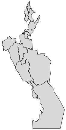
Mathematica graphics

What I have is the polygon for each subdivision, as above. What I want to get is the outline of the whole country, as below:
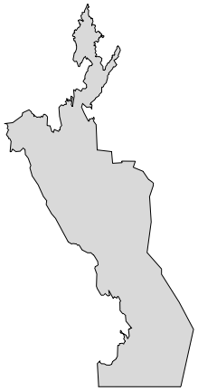
Mathematica graphics

How can I get the big outline starting with the outlines of the individual subdivisions?

The problem is that in my data the subdivision outlines do not fit perfectly because they have been simplified slightly to reduce the number of data points. Thus if I try BoundaryDiscretizeGraphics[Graphics[polygons]], I get the error

BoundaryMeshRegion::binsect: The boundary curves self-intersect or cross each other in ...

It is important that the result should be in the same coordinate system as the input data. The result should be in vector format (polygon or region). A small loss of precision is acceptable.


Below you'll find the code to artificially generate sample data that has this difficulty.

poly = #["Polygon"] & /@ CountryData["Uzbekistan"]["AdministrativeDivisions"] /. GeoPosition -> Identity;

spoly = poly /. Polygon[{line_}] :> Polygon@SimplifyLine[line, 0.01];

Graphics[spoly]

Mathematica graphics

Update: An alternative problem dataset, without the need to run simplification: spoly = #["Polygon"] & /@ CountryData["Chad"]["AdministrativeDivisions"] /. GeoPosition -> Identity;

SimplifyLine is a simple implementation of the Ramer-Douglas-Peucker algorithm that I use here to artificially create the difficulty I have in my actual data (which unfortunately I cannot post). Code is below:

rot[{x_, y_}] := {y, -x}

Options[SimplifyLine] = {Method -> "RamerDouglasPeucker"}

SimplifyLine::method = "Unknown method: ``.";

SimplifyLine[points_, threshold_, opt : OptionsPattern[]] :=
    With[{method = OptionValue[Method]},
      Switch[method,
        "RamerDouglasPeucker", rdp[DeleteDuplicates[points, #1 == #2 &], threshold],
        _, Message[SimplifyLine::method, method]; $Failed
      ]
    ]

rdp[{p1_, p2_}, _] := {p1, p2}
rdp[points_, th_] :=
    Module[{p1 = First[points], p2 = Last[points], b, dist, maxPos},
      b = Normalize@rot[p2 - p1];
      dist = Abs[b.(# - p1) & /@ points];
      maxPos = First@Ordering[dist, -1];
      If[
        dist[[maxPos]] < th
        ,
        {p1, p2},
        rdp[points[[;; maxPos]], th] ~Join~ Rest@rdp[points[[maxPos ;;]], th]
      ]
    ]
$\endgroup$
3
  • $\begingroup$ Sorry to comment outside the context of the question, can you let me know what is the meaning of SimplifyLine::method = "Unknown method: ``."; and its usage in Message[SimplifyLine::method, method]; or direct me to any source that can help me understand this. thank you $\endgroup$ Commented Dec 23, 2015 at 2:43
  • $\begingroup$ @Algohi It just issues a message. The last part of this tutorial deals with how to set up your own messages. $\endgroup$
    – Szabolcs
    Commented Dec 23, 2015 at 8:11
  • $\begingroup$ I'm guessing you've already seen Mark's implementation of Douglas-Peucker here? $\endgroup$ Commented Sep 10, 2017 at 17:40

3 Answers 3

13
$\begingroup$

The issue with BoundaryDiscretizeGraphics[Graphics[polygons]] can sometimes be resolved by discretizing each polygon individually and taking the RegionUnion.

RegionUnion[BoundaryDiscretizeGraphics /@ spoly]

However for the Chad polygons there is a problem - BoundaryDiscretizeGraphics doesn't like some of them and returns unevaluated. I don't understand the reason for this, but it appears that rounding the coordinates helps. You can then use this to find the outer boundary.

spoly = #["Polygon"] & /@ 
    CountryData["Chad"]["AdministrativeDivisions"] /. 
   GeoPosition -> Identity;

spoly = spoly /. x_Real :> Round[x, 0.0001];

br = RegionUnion[BoundaryDiscretizeGraphics /@ spoly];

merged = MeshRegion[MeshCoordinates[br], 
   br["IndexedBoundaryPolygons"][[br["BoundaryGroups"][[All, 1]]]]];

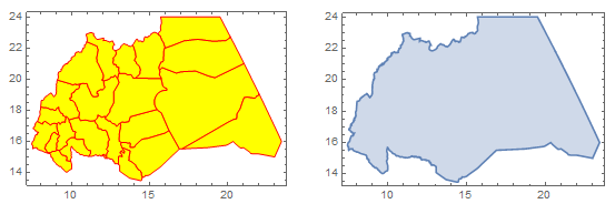
GraphicsRow[{Graphics[{Yellow, EdgeForm[Red], spoly}, Frame -> True], 
  RegionPlot[merged, AspectRatio -> Automatic]}]

enter image description here

The hack with Round is rather unsatisfactory, of course. Hopefully someone can explain what causes BoundaryDiscretizeGraphics to fail on some polygons and provide a better fix.

$\endgroup$
4
  • $\begingroup$ The failure of BoundaryDiscretizeGraphics to cooperate with the 3rd and 15th polygon is rather mysterious indeed. For #3 I thought it might be the south-most region where the border is drawn very strangely (and probably incorrectly), but removing this part makes no difference. Removing numbers 3 and 15 from the list (RegionUnion[BoundaryDiscretizeGraphics /@ spoly[[Complement[Range@Length@spoly, {3, 15}]]]], where spoly is the one above without Round) makes the kernel crash. [cont'd] $\endgroup$ Commented Dec 22, 2015 at 17:05
  • $\begingroup$ ... I noticed that each of the polygons has a list of lists of coordinates as argument (i.e., {{{x1,y1},{x2,y2},...{xn,yn}}}) which is an acceptable syntax that can be used to pass various (possibly disjunct) polygons to a single Polygon function. Removing the outer pair of curly brackets yields polygons that can still be drawn and on which BoundaryDiscretizeGraphics does work. However, RegionUnion doesn't seem to like working on those: RegionUnion[BoundaryDiscretizeGraphics[Polygon[#[[1, 1]]]] & /@ spoly] yields this. Looks buggy to me. $\endgroup$ Commented Dec 22, 2015 at 17:05
  • $\begingroup$ Interesting this: you really should study the output of InputForm[ BoundaryDiscretizeGraphics@Polygon[{{{0, 0}, {1, 1}, {2, 0}, {#, 0}}}]] & /@ {10^-5, 10^-11, 10^-12}. $\endgroup$ Commented Dec 22, 2015 at 21:18
  • $\begingroup$ Also very interesting and revealing: BoundaryDiscretizeGraphics@ Polygon[{{{0, 0}, {1, 1}, {1, 1} + {#, 0}, {2, 0}}}] & /@ {10^-5, 10^-11, 10^-13} $\endgroup$ Commented Dec 22, 2015 at 21:19
13
$\begingroup$

enter image description here

As I already pointed out in chat and similar to @Kuba's solution, a reasonably simple approach is to render the set of outlines as polygons. Due to the image grid, small differences at the borders are closed. And even if not, there exist many image filters to close gaps.

Once you have rendered the outlines, you are stuck with image pixel coordinates and you lost your original coordinate system, but with storing the original plot-range, this coordinate transformation can be reversed.

One of the important steps when you have your outlines as binary image is to get an ordered list of boundary pixel coordinates. To my knowledge, no built-in Mathematica routine exist that does exactly (and only) this. There are imperfect solutions like FindCurvePath or things like FindShortestTour, but these lack of an important thing: They don't know about image pixels, their neighborhood and that we have a solid object. What they do is trying to find a path based on a set of points, which is a harder problem.

Therefore, let me give an implementation of an algorithm that can be found in [Gonzalez & Woods] in chapter 11.1 which works directly on the image pixels and traces the boundary around the object.

This algorithm works by starting at the uppermost, leftmost object-pixel b0. This object-pixel's left neighbor is obviously a background pixel c0. From this neighbor, we go clockwise through all other neighbors n1, n2, ... of b0 until we find another object-pixel b1. The neighbor before b1 was of course a background-pixel that we set to c1.

This is basically, the iteration step. We start with a pair (b,c) and calculate the next pair by the above description. In Mathematica I can describe the iteration through all 8 neighbors by a repeated rotation:

NestList[
 Round[{{1/Sqrt[2], 1/Sqrt[2]}, {-(1/Sqrt[2]), 1/Sqrt[2]}}.#] &, 
  {-1, 0}, 8]
(* {{-1, 0}, {-1, 1}, {0, 1}, {1, 1}, 
   {1, 0}, {1, -1}, {0, -1}, {-1, -1}, {-1, 0}} *)

Therefore, a function that takes {{bx,by}, {cx,cy}} where b is the object pixel and c its background-neighbor, and a set of all object-positions pts could look like this

With[{rot = {{1/Sqrt[2], 1/Sqrt[2]}, {-(1/Sqrt[2]), 1/Sqrt[2]}}},
 nextPairC = Compile[{{p, _Integer, 2}, {pts, _Integer, 2}},
   Module[{n0 = Plus @@ ({1, -1}*Reverse[p]), n1 = {0, 0}, 
     b = First[p]},
    Do[
     n1 = Round[rot.n0];
     If[MemberQ[pts, b + n1],
      Break[];
      ];
     n0 = n1, {8}
     ];
    {n1 + b, n0 + b}
    ]
   ]
 ]

Since this is the core of the algorithm, the rest is a short wrapper around this. In the following, we use NestWhileList to repeatedly apply nextPairC until we reach the starting point. Exactly, the stop-condition reads: do until we reach an object point that is equal to b0 and its next object neighbor is equal to b1:

MooreBoundaryTracking[img_Image] := Module[{
   pixel = PixelValuePositions[img, 1], 
   p0, p1
  },
  p0 = {#, # - {1, 0}} &[First[SortBy[pixel, {Last, First}]]];
  p1 = nextPairC[p0, pixel];
  NestWhileList[
    nextPairC[#, pixel] &, 
    p1, 
    #1[[1]] != First[p0] && #2[[1]] != First[p1] &,
    2,
    10^5][[All, 1]]
 ]

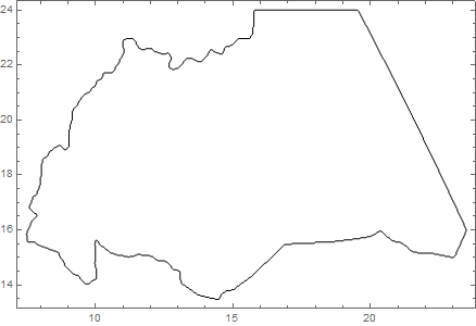
The method runs about 2 seconds for image-sizes of about 1000 pixel. With spoly as defined in Szabolcs question:

img = Rasterize[Graphics[spoly]] // ColorNegate // Binarize;
Graphics[Line@MooreBoundaryTracking[img]]
$\endgroup$
1
  • 2
    $\begingroup$ Guys, please give me a million upvotes if you like, but don't forget to upvote Simon and Kuba, because my answer only answers a small sub-problem, while theirs give a solution for the whole question! $\endgroup$
    – halirutan
    Commented Dec 22, 2015 at 16:19
12
$\begingroup$

Not sure what an outline really is so maybe:

Composition[

   Graphics[GraphicsComplex[#, Line@Last@FindShortestTour@#], Frame -> True] &

  , Function[image,
       Transpose @ MapThread[
            Rescale[#, {#2, #3}, {##4}] &, 
            {Transpose[#], {0., 0.}, ImageDimensions@image, 
             Sequence @@ Transpose@{{5, 25}, {13, 25}}}
        ] & @ PixelValuePositions[image, 1]
    ]

  ,  Binarize
  , Thinning
  , EdgeDetect
  , Binarize
  , ColorNegate
  , Rasterize[#, ImageSize -> 500] &

  ] @ Graphics[
  spoly,
  PlotRange -> {{5, 25}, {13, 25}},
  ImageMargins -> 0]

enter image description here

$\endgroup$
5
  • $\begingroup$ Thanks! This is halfway there. What's missing is the ordering of the boundary points. In other words, I would like a Polygon as the output. Based on another post (see chat), FindShortestTour will often work for getting the right ordering. (FindCurvePath will not). Handling shapes with holes in them (i.e. not singly connected) is more trouble, but I didn't mention that intentionally: I might be able to work around that. $\endgroup$
    – Szabolcs
    Commented Dec 22, 2015 at 11:51
  • $\begingroup$ Can you add the FindShortestTour and make it into a Polygon? $\endgroup$
    – Szabolcs
    Commented Dec 22, 2015 at 11:52
  • $\begingroup$ @Szabolcs Yep, I skipped it thinking maybe there is a faster method for such "obvious" and dense set. $\endgroup$
    – Kuba
    Commented Dec 22, 2015 at 11:57
  • $\begingroup$ For this data, FindShortestTour returns the result instantaneously and the result is good. Going to test for more complex cases soon. I think that for such cases fast heuristics will usually return the best solution (shortest tour). $\endgroup$
    – Szabolcs
    Commented Dec 22, 2015 at 12:00
  • $\begingroup$ @Szabolcs Ok, done. Good luck. $\endgroup$
    – Kuba
    Commented Dec 22, 2015 at 12:06

Your Answer

By clicking “Post Your Answer”, you agree to our terms of service and acknowledge you have read our privacy policy.

Not the answer you're looking for? Browse other questions tagged or ask your own question.