2
$\begingroup$

This is the continuation on my previous question Why does the minimum eigenvalue change dramatically when one basis function is added to the basis set?

Brief description of the problem: I would like to find excited states of this system: $$H=-\frac{1}{2}\Delta-\frac{1}{r}+\frac{25}{8}\rho^2-5/2$$where $r=(\rho,z,\phi)$ is a coordinate in the cylindrical system. The basis functions have the following form: $\psi_j=e^{-b_{j} z^2}e^{-a_{j} \rho^2}$, where $a_{j}$ and $b_{j}$ are parameters.

The energy of the ground state $(E_{min}=-1.3803982710899914)$ was found by @Alex Trounev using variational approach and this value is in excellent agreement with data from the literature (see this answer). The energies of excited states for this system are also known from the literature: $E_{1}=-0.193746$ (the first excited state), $E_{2}=-0.07365$ (the second excited state), $E_{3}=-0.03835$ (the third excited state), etc.

To find the excited states, @Alex Trounev suggested using a penalty method described here https://arxiv.org/pdf/2009.13556.pdf .

Let's start by finding the first excited state ($|\Psi_1\rangle$):

Following the article, the first excited state can be found as follows: $|\Psi_1\rangle=\operatorname{argmin} (O[\Psi_1])$ (formula 1 in the article), where $O[\Psi_1]$ is the objective functional. The objective functional has the following form: $O[\Psi_1]=E[\Psi_1]+\lambda_0|\vec{S}_0-\vec{S}_0^*|^2$ (formula 7 in the article), where $S_0=\frac{\langle\Psi_1|\Psi_0\rangle}{\sqrt{\langle\Psi_1|\Psi_1\rangle\langle\Psi_0|\Psi_0\rangle}}$ (formula 8 in the article), and $\vec{S}_0^ * $ is a set of target overlaps (If I understand correctly, in our case it is equal to 0).

Table 1 of the article shows the scheme of actions for finding excited states. In order to get the values from this scheme, let's turn to section II B of the article.

First of all, let's write the ground state function $|\Psi_0\rangle$, which is the anchor function in this problem. It was found in the previous question.

In the code I renamed $\rho\equiv r$ for convenience.

The ground state:

In[154]:= ClearAll["Global`*"]
al = {1.25, 1.25003, 1.25006, 1.251393, 1.252726, 1.2587955, 1.264865, 1.260499, 1.303186, 1.546232, 2.337185, 4.507307, 9.426298, 20.270036, 43.977048, 95.675215, 208.32642, 453.736619, 988.32236, 2152.803005, 4689.357171, 10214.647096};
bl = {0.026284, 0.0417685, 0.057253, 0.090983, 0.124713, 0.1981855, 0.271658, 0.417292, 0.61588, 1.008925, 1.949878, 4.24735, 9.251849, 20.15297, 43.898488, 95.622497, 208.291042, 453.712878`, 988.306428, 2152.792314, 4689.349997, 10214.642282};
cl = {0.006523295622643919`, -0.06054266302240082`, 0.14648250087347384`, -0.3150221502945908`, 0.416620632871218`, -0.3601131808535824`, 0.3912230593543366`, 
   0.012038542224830733`, 0.16818770546793724`, 0.17778604904585182`, 0.1738326674769321`, 0.12492347058872014`, 0.08226422142736733`, 0.05675211101544814`, 0.03735559092913218`, 0.026154779461694356`, 0.016669555882257724`, 0.01271934679906752`, 0.006364816098521608`,
    0.00797395974846925`, -0.0001602541764108519`, 0.006595023995239419`};
nmax = Length[al];
(*the basis function*)
a[j_] := al[[j]];
b[j_] := bl[[j]];
Psi[r_, z_, j_] := Exp[-b[j]*z^2]*Exp[-a[j]*r^2];
(*the ground state function*)
c[j_] := cl[[j]];
Psi0[r_, z_] = Sum[c[j]*Psi[r, z, j], {j, 1, nmax}]

Formula 9 from the article:

(*the 1st excited state*)
(*the basis function*)
Psi1[r_, z_, j_] := Exp[-b1[j]*z^2]*Exp[-a1[j]*r^2];
(*ρ0=|Psi0(|^2)+|Psi1(|^2)(formula 9 in the article)*)
Psi02[r_, z_] := 
  Sum[c[l1] *c[l2]*Psi[r, z, l1]*Psi[r, z, l2] , {l1, nmax}, {l2, 
    nmax}];
Psi12[r_, z_] := 
  Sum[c1[l1] *c1[l2]*Psi1[r, z, l1]*Psi1[r, z, l2] , {l1, nmax}, {l2, 
    nmax}];
ρ0[r_, z_] := Psi02[r, z] + Psi12[r, z]

Relative normalization (formula 11 and 10 in the article):

N0 = NIntegrate[
  Psi02[r, z]/ρ0[r, z]*r*2 Pi, {r, 0, Infinity}, {z, -Infinity, Infinity}]

There are 66 parameters (a1[j], b1[j] and c1[j]) in the problem (with the current choice of the excited state function structure). In order to find the derivative with respect to each parameter for relative normalization, the authors give formula 12:

Psi11[r_, z_] := Sum[c1[l] *Psi1[r, z, l] , {l, nmax}];
da1N0 = 2*
   Re[NIntegrate[(
      E^(-r^2 a1[1] - z^2 b1[1]) *(-r^2)*c1[1]*Psi11[r, z])/ρ0[r,
        z]*r*2 Pi, {r, 0, Infinity}, {z, -Infinity, Infinity}]];
db1N0 = 2*
   Re[NIntegrate[(
      E^(-r^2 a1[1] - z^2 b1[1]) *(-z^2)*c1[1]*Psi11[r, z])/ρ0[r,
        z]*r*2 Pi, {r, 0, Infinity}, {z, -Infinity, Infinity}]];
dc1N0 = 2*
   Re[NIntegrate[(
      E^(-r^2 a1[1] - z^2 b1[1]) *(-r^2)*Psi11[r, z])/ρ0[r, z]*
      r*2 Pi, {r, 0, Infinity}, {z, -Infinity, Infinity}]];

A few questions:

  1. I took a certain set of numbers as parameters of the excited wave function (Psi11) and checked the calculations of the normalization factor and its derivatives, Mathematica gives errors. Is it due to the fact that I misunderstand the formulas from the article?

  2. The scheme shown in Table 1 (in the article) is not very clear, especially points (c)–(i). If you could write these points more simply, it would help me a lot.

I would be glad to any comments on solving the problem.
I am sorry for the not quite typical question, but in the context of my previous questions, which make up the topic series, finding a solution to this problem is of interest.

$\endgroup$
4
  • $\begingroup$ @Alex Trounev, your comments are needed ) $\endgroup$
    – Mam Mam
    Commented May 9, 2023 at 6:01
  • 1
    $\begingroup$ Mathematica gives errors. What are they? $\endgroup$
    – Ghoster
    Commented May 9, 2023 at 6:15
  • $\begingroup$ @Ghoster, errors of this type evaluated to Overflow, Indeterminate, or Infinity for all sampling points in the region with boundaries {{3.,1.},{0.,352422.}}. I just tried to check these formulas with certain given parameters, the correct values of which should be found later from minimization (penalty method). $\endgroup$
    – Mam Mam
    Commented May 9, 2023 at 6:28
  • $\begingroup$ "In the code I renamed rho to r. " The Hamiltonian in the first line is defined with rho the plane radius, while 1/r is the spherical Coulomb potential. Your problem is not existent, neither in mathematics nor in physics. $\endgroup$
    – Roland F
    Commented May 9, 2023 at 20:39

2 Answers 2

1
$\begingroup$

To compute exited states we can use the penalty method as follows. Note that any exited state wave function is orthogonal to the ground state, therefore $\langle\Psi_1|\Psi_0\rangle=0$. We use this equation as constraint for minimization problem. First we compute ground state

a0j = {1.25, 1.25003, 1.25006, 1.251393, 1.252726, 1.2587955, 
   1.264865, 1.260499, 1.303186, 1.546232, 2.337185, 4.507307, 
   9.426298, 20.270036, 43.977048, 95.675215, 208.32642, 453.736619, 
   988.32236, 2152.803005, 4689.357171, 10214.647096};

b0j = {0.026284, 0.0417685, 0.057253, 0.09098300000000001, 0.124713, 
   0.19818550000000001, 0.271658, 0.417292, 0.61588, 1.008925, 
   1.949878, 4.24735, 9.251849, 20.15297, 43.898488, 95.622497, 
   208.291042, 453.712878`, 988.306428, 2152.792314, 4689.349997, 
   10214.642282};
nmax = Length[a0j]; var = 
 Join[Table[a[n], {n, nmax}], Table[b[n], {n, nmax}], 
  Table[c[n], {n, nmax}]];
Psi[r_, z_, j_] := Exp[-b[j]*z^2]*Exp[-a[j]*r^2];


(*kinetic energy*)
Kk[r_, z_, n1_, n2_] := 
  FullSimplify[
   Psi[r, z, n2]*
    Laplacian[Psi[r, z, n1], {r, \[Theta], z}, "Cylindrical"]];

ss = Integrate[
  Kk[r, z, l1, l2] r, {r, 0, \[Infinity]}, {z, -Infinity, Infinity}, 
  Assumptions -> {a[l1] > 0, b[l1] > 0, a[l2] > 0, b[l2] > 0}];
Kx = -1/2 2 Pi Sum[c[l1] c[l2] ss, {l1, nmax}, {l2, nmax}]


(*potential energy*)
VP1[r_, z_] := -1/Sqrt[r^2 + z^2] + 25/8 r^2 - 5/2;

Px = Integrate[
  Psi[r, z, l2]*VP1[r, z]*Psi[r, z, l1]*r , {r, 
   0, \[Infinity]}, {z, -Infinity, Infinity}, 
  Assumptions -> {a[l1] > 0, b[l1] > 0, a[l2] > 0, b[l2] > 0}];

Px = 2 Pi Sum[c[l1] c[l2] Px, {l1, nmax}, {l2, nmax}];


int = Integrate[
  Psi[r, z, l1] Psi[r, z, l2] r , {r, 0, \[Infinity]}, {z, -Infinity, 
   Infinity}, 
  Assumptions -> {a[l1] > 0, b[l1] > 0, a[l2] > 0, b[l2] > 0}];
norm = {2 Pi Sum[c[l1] c[l2] int, {l1, nmax}, {l2, nmax}] == 
   1}; cons = 
 Join[Table[a[n] == a0j[[n]], {n, nmax}], 
  Table[b[n] == b0j[[n]], {n, nmax}], norm];


sol = NMinimize[{Kx + Px, cons}, var, 
   Method -> "DifferentialEvolution"]; 

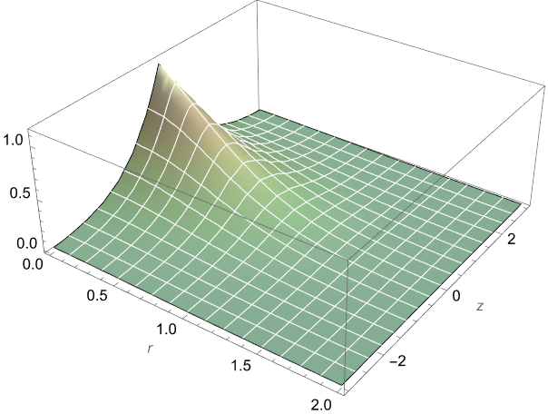
The ground state energy is sol[[1]]= -1.3803982710899914, the ground state wave function $\Psi_0=\sum_j c_j\Psi(r,z,j)$ is given by

\[Psi]0 = Sum[c[j] Psi[r, z, j], {j, 1, nmax}] /. sol[[2]];

Plot3D[\[Psi]0, {r, 0, 2}, {z, -3, 3}, PlotRange -> All, 
  ColorFunction -> "ArmyColors", MeshStyle -> White, 
  AxesLabel -> Automatic] // Quiet 

Figure 1

Second step, to compute first exited state we use

Do[c0[j] = c[j] /. sol[[2]];, {j, 1, nmax}]; ps10 = 
 Integrate[
  Psi[r, z, l2] Psi[r, z, l1]*r , {r, 0, \[Infinity]}, {z, -Infinity, 
   Infinity}, 
  Assumptions -> {a[l1] > 0, b[l1] > 0, a[l2] > 0, b[l2] > 0}];

pen = (Sum[c0[l1] c[l2] ps10, {l1, nmax}, {l2, nmax}])^2;

cons1 = Join[Table[a[n] == a0j[[n]], {n, nmax}], 
  Table[b[n] == b0j[[n]], {n, nmax}], norm, {pen == 0}]; sol1 = 
 NMinimize[{Kx + Px, cons1}, var, Method -> "DifferentialEvolution"] 

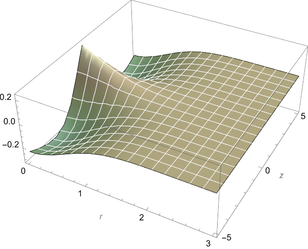
The first exited state energy is sol1[[1]]=-0.1936924825598707, the first exited state wave function $\Psi_1=\sum_j c_j\Psi(r,z,j)$ is given by

\[Psi]1 = Sum[c[j] Psi[r, z, j], {j, 1, nmax}] /. sol1[[2]];

Visualization

Plot3D[\[Psi]1, {r, 0, 3}, {z, -5, 5}, PlotRange -> All, 
  ColorFunction -> "ArmyColors", MeshStyle -> White, 
  AxesLabel -> Automatic] // Quiet

Figure 2

Update 1. To compute ground and exited states we use model described in the paper Accurate and balanced anisotropic Gaussian type orbital basis sets for atoms in strong magnetic fields. They propose basis functions in the form $\psi_j=\rho^{n_{\rho j}}z^{n_{zj}}e^{-a_j\rho^2-b_j z^2 +i m_j \phi }$ where parameters $a_j, b_j, n_{\rho j}, n_{zj}$ can be calculated with C utility available to download from here. Example of usage for hydrogen atoms in magnetic field B = 1.0 a.u. with electron on $s$ or $p_0$ orbitals. The ground state computation not so differ from above

base = {{0, 0, 0.251400, 0.026284}, {0, 0, 0.258885, 0.057253}, {0, 
    0, 0.257760, 0.086129}, {0, 0, 0.261516, 0.127117}, {0, 0, 
    0.291075, 0.187611}, {0, 0, 0.387437, 0.313972}, {0, 0, 0.720180, 
    0.676716}, {0, 0, 1.499564, 1.474065}, {0, 0, 3.225863, 
    3.210904}, {0, 0, 7.002972, 6.994196}, {0, 0, 15.240353, 
    15.235205}, {0, 0, 33.189319, 33.186299}, {0, 0, 72.290292, 
    72.288520}, {0, 0, 157.464519, 157.463480}, {0, 0, 342.997640, 
    342.997030}, {0, 0, 747.138440, 747.138082}, {0, 0, 1627.464197, 
    1627.463987}};
a0j = base[[All, 3]]; b0j = base[[All, 4]];

VP1[r_, z_] := -1/Sqrt[r^2 + z^2] + 1/8 r^2 - 1/2;

nmax = Length[a0j]; var = 
 Join[Table[a[n], {n, nmax}], Table[b[n], {n, nmax}], 
  Table[c[n], {n, nmax}]];
Psi[r_, z_, j_] := Exp[-b[j]*z^2]*Exp[-a[j]*r^2];


(*kinetic energy*)
Kk[r_, z_, n1_, n2_] := 
  FullSimplify[
   Psi[r, z, n2]*
    Laplacian[Psi[r, z, n1], {r, \[Theta], z}, "Cylindrical"]];

ss = Integrate[
   Kk[r, z, l1, l2] r, {r, 0, \[Infinity]}, {z, -Infinity, Infinity}, 
   Assumptions -> {a[l1] > 0, b[l1] > 0, a[l2] > 0, b[l2] > 0}];
Kx = -1/2 2 Pi Sum[c[l1] c[l2] ss, {l1, nmax}, {l2, nmax}];


(*potential energy*)
Px = Integrate[
   Psi[r, z, l2]*VP1[r, z]*Psi[r, z, l1]*r, {r, 
    0, \[Infinity]}, {z, -Infinity, Infinity}, 
   Assumptions -> {a[l1] > 0, b[l1] > 0, a[l2] > 0, b[l2] > 0}];

Px = 2 Pi Sum[c[l1] c[l2] Px, {l1, nmax}, {l2, nmax}];


int = Integrate[
   Psi[r, z, l1] Psi[r, z, l2] r, {r, 0, \[Infinity]}, {z, -Infinity, 
    Infinity}, 
   Assumptions -> {a[l1] > 0, b[l1] > 0, a[l2] > 0, b[l2] > 0}];
norm = {2 Pi Sum[c[l1] c[l2] int, {l1, nmax}, {l2, nmax}] == 
   1}; cons = 
 Join[Table[a[n] == a0j[[n]], {n, nmax}], 
  Table[b[n] == b0j[[n]], {n, nmax}], norm];


sol = NMinimize[{Kx + Px, cons}, var, 
   Method -> "DifferentialEvolution"];

The ground state energy is sol[[1]]=-0.8311682094831563, while form the paper linked we have -0.83116821. To compute energy of p0 state we have to join two basis and put $n_{zj}=1$ for this case:

base0 = {{0, 0, 0.251400, 0.026284}, {0, 0, 0.258885, 0.057253}, {0, 
    0, 0.257760, 0.086129}, {0, 0, 0.261516, 0.127117}, {0, 0, 
    0.291075, 0.187611}, {0, 0, 0.387437, 0.313972}, {0, 0, 0.720180, 
    0.676716}, {0, 0, 1.499564, 1.474065}, {0, 0, 3.225863, 
    3.210904}, {0, 0, 7.002972, 6.994196}, {0, 0, 15.240353, 
    15.235205}, {0, 0, 33.189319, 33.186299}, {0, 0, 72.290292, 
    72.288520}, {0, 0, 157.464519, 157.463480}, {0, 0, 342.997640, 
    342.997030}, {0, 0, 747.138440, 747.138082}, {0, 0, 1627.464197, 
    1627.463987}};

(*H2p0_B1.bas,energy=-0.2600041,-0.26000662*)
base1 = {{0, 1, 0.250013, 0.012066}, {0, 1, 0.250572, 0.026284}, {0, 
    1, 0.253650, 0.057253}, {0, 1, 0.257357, 0.090961}, {0, 1, 
    0.281270, 0.144874}, {0, 1, 0.373903, 0.267507}, {0, 1, 0.679589, 
    0.582700}, {0, 1, 1.366163, 1.269275}, {0, 1, 2.861704, 
    2.764815}, {0, 1, 6.119386, 6.022497}, {0, 1, 13.215477, 
    13.118589}, {0, 1, 28.672638, 28.575749}};


base = Join[base0, base1]; a0j = base[[All, 3]]; b0j = base[[All, 4]];

VP1[r_, z_] := -1/Sqrt[r^2 + z^2] + 1/8 r^2 - 1/2;

nmax = Length[a0j]; var = 
 Join[Table[a[n], {n, nmax}], Table[b[n], {n, nmax}], 
  Table[c[n], {n, nmax}]];
Psi[r_, z_, j_] := z Exp[-b[j]*z^2]*Exp[-a[j]*r^2];
(*kinetic energy*)
Kk[r_, z_, n1_, n2_] := 
  FullSimplify[
   Psi[r, z, n2]*
    Laplacian[Psi[r, z, n1], {r, \[Theta], z}, "Cylindrical"]];

ss = Integrate[
   Kk[r, z, l1, l2] r, {r, 0, \[Infinity]}, {z, -Infinity, Infinity}, 
   Assumptions -> {a[l1] > 0, b[l1] > 0, a[l2] > 0, b[l2] > 0}];
Kx = -1/2 2 Pi Sum[c[l1] c[l2] ss, {l1, nmax}, {l2, nmax}];
(*potential energy*)
Px = Integrate[
   Psi[r, z, l2]*VP1[r, z]*Psi[r, z, l1]*r, {r, 
    0, \[Infinity]}, {z, -Infinity, Infinity}, 
   Assumptions -> {a[l1] > 0, b[l1] > 0, a[l2] > 0, b[l2] > 0}];

Px = 2 Pi Sum[c[l1] c[l2] Px, {l1, nmax}, {l2, nmax}];


int = Integrate[
   Psi[r, z, l1] Psi[r, z, l2] r, {r, 0, \[Infinity]}, {z, -Infinity, 
    Infinity}, 
   Assumptions -> {a[l1] > 0, b[l1] > 0, a[l2] > 0, b[l2] > 0}];
norm = {2 Pi Sum[c[l1] c[l2] int, {l1, nmax}, {l2, nmax}] == 
   1}; cons = 
 Join[Table[a[n] == a0j[[n]], {n, nmax}], 
  Table[b[n] == b0j[[n]], {n, nmax}], norm];


sol = NMinimize[{Kx + Px, cons}, var, 
   Method -> "DifferentialEvolution"]; 

The energy of p0 state is sol[[1]]=-0.26000636548224826 that is in a good agreement with energy=-0.2600041 from the paper.

$\endgroup$
6
  • $\begingroup$ Thank you very much for the explanation! This is a great answer, It is very helpful $\endgroup$
    – Mam Mam
    Commented May 9, 2023 at 13:17
  • $\begingroup$ Now I'm trying to get the second excited state by analogy and I get a very interesting situation. Due to the fact that not only the second excited state is orthogonal to the first, but also the ground state is orthogonal to the first excited state, it turns out that the minimization returns to the ground state again (because it is below the second excited level and is also orthogonal to the first excited level). In order to avoid this, it is necessary to write an additional condition into cons2? $\endgroup$
    – Mam Mam
    Commented May 9, 2023 at 13:38
  • $\begingroup$ There is a typo in the answer, a line Kx = -1/2 2 Pi Sum[c[l1] c[l2] ss, {l1, nmax}, {l2, nmax}]; from the previous answer (mathematica.stackexchange.com/questions/284809/…) is missing here. $\endgroup$
    – Mam Mam
    Commented May 9, 2023 at 15:47
  • 1
    $\begingroup$ Yes, you are right. Try $\langle\Psi_2|\Psi_0\rangle=0$ and $\langle\Psi_2|\Psi_1\rangle=0$ for the second state. $\endgroup$ Commented May 9, 2023 at 15:50
  • $\begingroup$ Thanks a lot for the comment! $\endgroup$
    – Mam Mam
    Commented May 9, 2023 at 19:30
1
$\begingroup$

Following @Alex Trounev answer. Let's find the energy of the second excited state. Now it is necessary to take into account two conditions of orthogonality, since the second excited state is orthogonal to the ground state $<\Psi_2|\Psi_0>=0$, as well as to the first excited state $<\Psi_2|\Psi_1>=0$.

Do[c1[j] = c[j] /. sol1[[2]];, {j, 1, nmax}];
ps21 = Integrate[
   Psi[r, z, l2] Psi[r, z, l1]*r, {r, 0, \[Infinity]}, {z, -Infinity, 
    Infinity}, 
   Assumptions -> {a[l1] > 0, b[l1] > 0, a[l2] > 0, b[l2] > 0}];
pen2 = (Sum[c1[l1] c[l2] ps21, {l1, nmax}, {l2, nmax}])^2;
cons2 = Join[Table[a[n] == a0j[[n]], {n, nmax}], 
   Table[b[n] == b0j[[n]], {n, nmax}], norm, {pen == 0}, {pen2 == 0}];
sol2 = NMinimize[{Kx + Px, cons2}, var, 
  Method -> "DifferentialEvolution"]
sol2[[1]]

Out[110]= {-0.0640854 + 0. I, {a[1] -> 1.25, a[2] -> 1.25003, 
  a[3] -> 1.25006, a[4] -> 1.25139, a[5] -> 1.25273, a[6] -> 1.2588, 
  a[7] -> 1.26487, a[8] -> 1.2605, a[9] -> 1.30319, a[10] -> 1.54623, 
  a[11] -> 2.33719, a[12] -> 4.50731, a[13] -> 9.4263, a[14] -> 20.27,
   a[15] -> 43.977, a[16] -> 95.6752, a[17] -> 208.326, 
  a[18] -> 453.737, a[19] -> 988.322, a[20] -> 2152.8, 
  a[21] -> 4689.36, a[22] -> 10214.6, b[1] -> 0.026284, 
  b[2] -> 0.0417685, b[3] -> 0.057253, b[4] -> 0.090983, 
  b[5] -> 0.124713, b[6] -> 0.198186, b[7] -> 0.271658, 
  b[8] -> 0.417292, b[9] -> 0.61588, b[10] -> 1.00893, 
  b[11] -> 1.94988, b[12] -> 4.24735, b[13] -> 9.25185, 
  b[14] -> 20.153, b[15] -> 43.8985, b[16] -> 95.6225, 
  b[17] -> 208.291, b[18] -> 453.713, b[19] -> 988.306, 
  b[20] -> 2152.79, b[21] -> 4689.35, b[22] -> 10214.6, 
  c[1] -> -10.0667, c[2] -> 43.2035, c[3] -> -59.4205, 
  c[4] -> 58.3119, c[5] -> -44.6414, c[6] -> 22.3368, 
  c[7] -> -12.8573, c[8] -> 5.01677, c[9] -> -2.6131, 
  c[10] -> 0.860936, c[11] -> -0.291487, c[12] -> 0.0832379, 
  c[13] -> -0.0671967, c[14] -> 0.0298749, c[15] -> -0.0317333, 
  c[16] -> 0.0168776, c[17] -> -0.0175496, c[18] -> 0.0100948, 
  c[19] -> -0.00949738, c[20] -> 0.00499179, c[21] -> -0.00346965, 
  c[22] -> 0.000418}}

Out[111]= -0.0640854 + 0. I

The value of the received energy ($E_2=-0.0640854$) is higher than the value from the literature ($E_2=-0,07365$).

Is this due to the fact that the considered number of basis functions (22) is not enough to describe the higher excited states?

Such a difference in energies is due to the mixing of levels. If only the third excited state is taken into account in mixing, then the expression for the second excited state will take the form: $|\Psi_2>=A_1|\Psi_{2, pure}>+A_2|\Psi_{3, pure}>$

$|\Psi_2>=A_1(c[1]_{2,\Psi_{pure}}|\Psi(\alpha_1,\beta_1)>+...)$+ $A_2(c[1]_{3,\Psi_{pure}}|\Psi(\alpha_1,\beta_1)>+...)$

$\endgroup$
22
  • 1
    $\begingroup$ It depends on method, but using orthogonalization and normalization only we can compute mixture of states as well. Let try FindMinimum with c2 computed above as starting point. $\endgroup$ Commented May 10, 2023 at 2:16
  • 1
    $\begingroup$ In this case mixing states is $\psi=\sum_{i=2}^{nmax}C_i \psi_i$, where $\psi_i$ is orthogonal to $\psi_0, \psi_1$. It is why we need some additional constraint to select exited states $\psi_i$. $\endgroup$ Commented May 10, 2023 at 13:11
  • 1
    $\begingroup$ Please, pay attention, that in a case of matrix method we need about 200 basis functions to compute first 10 eigenvalues with high accuracy - see my answer on mathematica.stackexchange.com/questions/200448/… . In this regards the optimization method working very good on 22 basis functions. $\endgroup$ Commented May 11, 2023 at 4:11
  • 1
    $\begingroup$ Actually, as I understand from the paper 'Accurate and balanced anisotropic Gaussian type orbital basis sets for atoms in strong magnetic fields' we need to use new basis functions for every orbitals. Therefore, our approach is good, but to compute $\Psi_2$ we need new basis. $\endgroup$ Commented May 11, 2023 at 6:03
  • 1
    $\begingroup$ This is very long time research starting from C. Aldrich and R. L. Greene, Phys. Status Solidi B 93, 343 (1979). On every step somebody added new correlation. Finally we have very complicated empirical model. There is C code to compute $a_j, b_j, n_{\rho j}, n_{zj}$ for base functions $\psi_j=\rho^{n_{\rho j}}z^{n_{zj}}e^{-a_j\rho^2-b_j z^2 +i m_j \phi }$. While we try to compute exited states using one base for ground state. :) $\endgroup$ Commented May 11, 2023 at 7:23

Your Answer

By clicking “Post Your Answer”, you agree to our terms of service and acknowledge you have read our privacy policy.

Not the answer you're looking for? Browse other questions tagged or ask your own question.