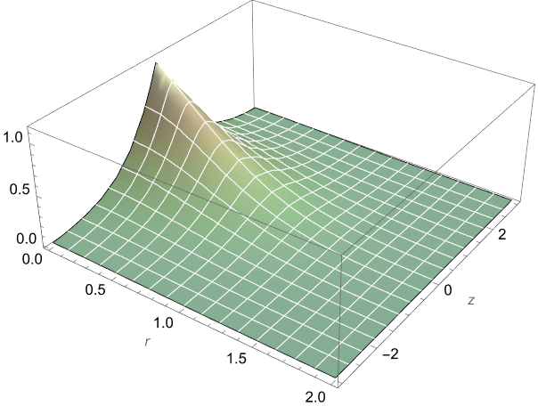
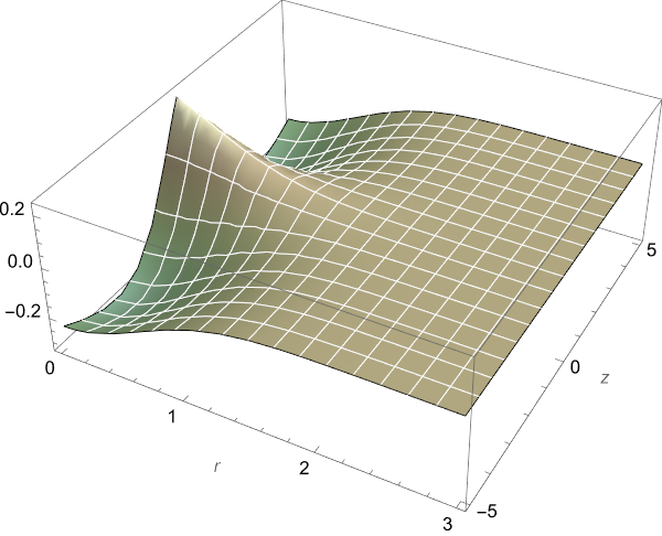
Update 1. To compute ground and exited states we use model described in the paper Accurate and balanced anisotropic Gaussian type orbital basis sets for atoms in strong magnetic fields. They propose basis functions in the form $\psi_j=\rho^{n_{\rho j}}z^{n_{zj}}e^{-a_j\rho^2-b_j z^2 +i m_j \phi }$ where parameters $a_j, b_j, n_{\rho j}, n_{zj}$ can be calculated with C utility available to download from here. Example of usage for hydrogen atoms in magnetic field B = 1.0 a.u. with electron on $s$ or $p_0$ orbitals. The ground state computation not so differ from above
base = {{0, 0, 0.251400, 0.026284}, {0, 0, 0.258885, 0.057253}, {0,
    0, 0.257760, 0.086129}, {0, 0, 0.261516, 0.127117}, {0, 0,
    0.291075, 0.187611}, {0, 0, 0.387437, 0.313972}, {0, 0, 0.720180,
    0.676716}, {0, 0, 1.499564, 1.474065}, {0, 0, 3.225863,
    3.210904}, {0, 0, 7.002972, 6.994196}, {0, 0, 15.240353,
    15.235205}, {0, 0, 33.189319, 33.186299}, {0, 0, 72.290292,
    72.288520}, {0, 0, 157.464519, 157.463480}, {0, 0, 342.997640,
    342.997030}, {0, 0, 747.138440, 747.138082}, {0, 0, 1627.464197,
    1627.463987}};
a0j = base[[All, 3]]; b0j = base[[All, 4]];

VP1[r_, z_] := -1/Sqrt[r^2 + z^2] + 1/8 r^2 - 1/2;

nmax = Length[a0j]; var =
 Join[Table[a[n], {n, nmax}], Table[b[n], {n, nmax}],
  Table[c[n], {n, nmax}]];
Psi[r_, z_, j_] := Exp[-b[j]*z^2]*Exp[-a[j]*r^2];


(*kinetic energy*)
Kk[r_, z_, n1_, n2_] :=
  FullSimplify[
   Psi[r, z, n2]*
    Laplacian[Psi[r, z, n1], {r, \[Theta], z}, "Cylindrical"]];

ss = Integrate[
   Kk[r, z, l1, l2] r, {r, 0, \[Infinity]}, {z, -Infinity, Infinity},
   Assumptions -> {a[l1] > 0, b[l1] > 0, a[l2] > 0, b[l2] > 0}];
Kx = -1/2 2 Pi Sum[c[l1] c[l2] ss, {l1, nmax}, {l2, nmax}];


(*potential energy*)
Px = Integrate[
   Psi[r, z, l2]*VP1[r, z]*Psi[r, z, l1]*r, {r,
    0, \[Infinity]}, {z, -Infinity, Infinity},
   Assumptions -> {a[l1] > 0, b[l1] > 0, a[l2] > 0, b[l2] > 0}];

Px = 2 Pi Sum[c[l1] c[l2] Px, {l1, nmax}, {l2, nmax}];


int = Integrate[
   Psi[r, z, l1] Psi[r, z, l2] r, {r, 0, \[Infinity]}, {z, -Infinity,
    Infinity},
   Assumptions -> {a[l1] > 0, b[l1] > 0, a[l2] > 0, b[l2] > 0}];
norm = {2 Pi Sum[c[l1] c[l2] int, {l1, nmax}, {l2, nmax}] ==
   1}; cons =
 Join[Table[a[n] == a0j[[n]], {n, nmax}],
  Table[b[n] == b0j[[n]], {n, nmax}], norm];


sol = NMinimize[{Kx + Px, cons}, var,
   Method -> "DifferentialEvolution"];
The ground state energy is sol[[1]]=-0.8311682094831563, while form the paper linked we have -0.83116821. To compute energy of p0 state we have to join two basis and put $n_{zj}=1$ for this case:
base0 = {{0, 0, 0.251400, 0.026284}, {0, 0, 0.258885, 0.057253}, {0,
    0, 0.257760, 0.086129}, {0, 0, 0.261516, 0.127117}, {0, 0,
    0.291075, 0.187611}, {0, 0, 0.387437, 0.313972}, {0, 0, 0.720180,
    0.676716}, {0, 0, 1.499564, 1.474065}, {0, 0, 3.225863,
    3.210904}, {0, 0, 7.002972, 6.994196}, {0, 0, 15.240353,
    15.235205}, {0, 0, 33.189319, 33.186299}, {0, 0, 72.290292,
    72.288520}, {0, 0, 157.464519, 157.463480}, {0, 0, 342.997640,
    342.997030}, {0, 0, 747.138440, 747.138082}, {0, 0, 1627.464197,
    1627.463987}};

(*H2p0_B1.bas,energy=-0.2600041,-0.26000662*)
base1 = {{0, 1, 0.250013, 0.012066}, {0, 1, 0.250572, 0.026284}, {0,
    1, 0.253650, 0.057253}, {0, 1, 0.257357, 0.090961}, {0, 1,
    0.281270, 0.144874}, {0, 1, 0.373903, 0.267507}, {0, 1, 0.679589,
    0.582700}, {0, 1, 1.366163, 1.269275}, {0, 1, 2.861704,
    2.764815}, {0, 1, 6.119386, 6.022497}, {0, 1, 13.215477,
    13.118589}, {0, 1, 28.672638, 28.575749}};


base = Join[base0, base1]; a0j = base[[All, 3]]; b0j = base[[All, 4]];

VP1[r_, z_] := -1/Sqrt[r^2 + z^2] + 1/8 r^2 - 1/2;

nmax = Length[a0j]; var =
 Join[Table[a[n], {n, nmax}], Table[b[n], {n, nmax}],
  Table[c[n], {n, nmax}]];
Psi[r_, z_, j_] := z Exp[-b[j]*z^2]*Exp[-a[j]*r^2];
(*kinetic energy*)
Kk[r_, z_, n1_, n2_] :=
  FullSimplify[
   Psi[r, z, n2]*
    Laplacian[Psi[r, z, n1], {r, \[Theta], z}, "Cylindrical"]];

ss = Integrate[
   Kk[r, z, l1, l2] r, {r, 0, \[Infinity]}, {z, -Infinity, Infinity},
   Assumptions -> {a[l1] > 0, b[l1] > 0, a[l2] > 0, b[l2] > 0}];
Kx = -1/2 2 Pi Sum[c[l1] c[l2] ss, {l1, nmax}, {l2, nmax}];
(*potential energy*)
Px = Integrate[
   Psi[r, z, l2]*VP1[r, z]*Psi[r, z, l1]*r, {r,
    0, \[Infinity]}, {z, -Infinity, Infinity},
   Assumptions -> {a[l1] > 0, b[l1] > 0, a[l2] > 0, b[l2] > 0}];

Px = 2 Pi Sum[c[l1] c[l2] Px, {l1, nmax}, {l2, nmax}];


int = Integrate[
   Psi[r, z, l1] Psi[r, z, l2] r, {r, 0, \[Infinity]}, {z, -Infinity,
    Infinity},
   Assumptions -> {a[l1] > 0, b[l1] > 0, a[l2] > 0, b[l2] > 0}];
norm = {2 Pi Sum[c[l1] c[l2] int, {l1, nmax}, {l2, nmax}] ==
   1}; cons =
 Join[Table[a[n] == a0j[[n]], {n, nmax}],
  Table[b[n] == b0j[[n]], {n, nmax}], norm];


sol = NMinimize[{Kx + Px, cons}, var,
   Method -> "DifferentialEvolution"];
The energy of p0 state is sol[[1]]=-0.26000636548224826 that is in a good agreement with energy=-0.2600041 from the paper.


