The direct problem to determine points {x1,x2} where restrictions $\nabla h1=\nabla h2=0$ are true has solution as follows:
w0 = 314.1593;
Pm = 1.2;
Pe = 1.6382;
Damp = 5;
TJ = 6;
eq = {w0*x2 + D[h1[x1, x2], x1]*(w0*x2) +
     D[h1[x1, x2], x2]*(Pm - Pe*Sin[x1] - Damp*x2)/TJ ==
    w0*(x2 + h2[x1, x2]), (Pm - Pe*Sin[x1] - Damp*x2)/TJ +
     D[h2[x1, x2], x1]*(w0*x2) +
     D[h2[x1, x2], x2]*(Pm - Pe*Sin[x1] - Damp*x2)/
       TJ == -(Pe^2 - Pm^2)^0.5/TJ*(x1 + h1[x1, x2]) -
     Damp/TJ*(x2 + h2[x1, x2])};
bc = DirichletCondition[{h1[x1, x2] == 0, h2[x1, x2] == 0}, x1 == -1];

s = NDSolve[{eq, bc}, {h1[x1, x2], h2[x1, x2]}, {x1, -1,
    4}, {x2, -0.04, 0.04}];
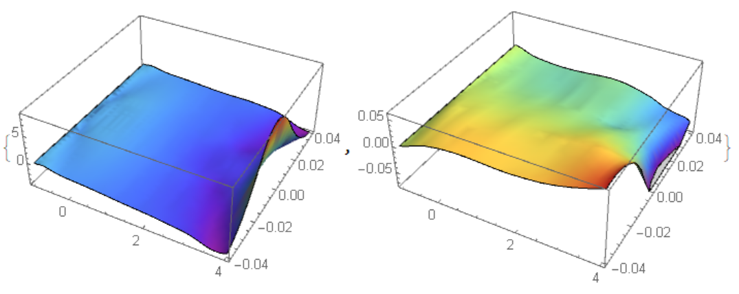
Visualization of numerical solution
{Plot3D[h1[x1, x2] /. s[[1]], {x1, -1, 4}, {x2, -0.04, 0.04},
  PlotRange -> All, Mesh -> None, ColorFunction -> "Rainbow"],
 Plot3D[h2[x1, x2] /. s[[1]], {x1, -1, 4}, {x2, -0.04, 0.04},
  ColorFunction -> "Rainbow", Mesh -> None]}
Now we are looking points where restrictions are true, for this we use
eq1 =
 eq /. {D[h1[x1, x2], x1] -> 0, D[h2[x1, x2], x2] -> 0,
   D[h1[x1, x2], x2] -> 0, D[h2[x1, x2], x1] -> 0}

Out[]= {0. + 314.159 x2 == 314.159 (x2 + h2[x1, x2]),
 0. + 1/6 (1.2 - 5 x2 - 1.6382 Sin[x1]) == -0.185869 (x1 +
      h1[x1, x2]) - 5/6 (x2 + h2[x1, x2])}
Then we solve eq1 using
Solve[eq1, {h1[x1, x2], h2[x1, x2]}]

Out[]= {{h1[x1, x2] -> -1.07603 - 1. x1 - 5.97316*10^-16 x2 +
    1.46896 Sin[x1], h2[x1, x2] -> 0.}}
This general solution can be plot with our numerical solution as
Show[ContourPlot[
  Evaluate[h2[x1, x2] == 0. /. s], {x1, -1, 4}, {x2, -0.04, 0.04}],
 ContourPlot[
  Evaluate[h1[x1, x2] == -1.076027972872623` - 1.` x1 -
      5.973155153119597`*^-16 x2 + 1.4689575209666093` Sin[x1] /.
    s], {x1, -1, 4}, {x2, -0.04, 0.04}, ContourStyle -> Red]]
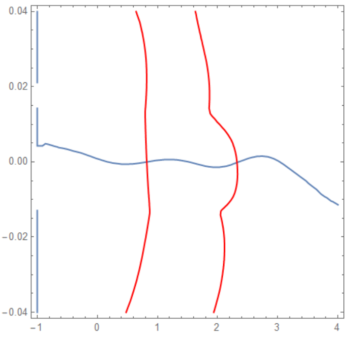
Points where gray and red lines crossing we can calculate with
FindRoot[{Evaluate[h2[x1, x2] == 0. /. s],
  h1[x1, x2] == -1.076027972872623` - 1.` x1 -
     5.973155153119597`*^-16 x2 + 1.4689575209666093` Sin[x1] /.
   s}, {{x1, 2.5}, {x2, 0}}]

Out[]= {x1 -> 2.32257, x2 -> -0.000184708}

 FindRoot[{Evaluate[h2[x1, x2] == 0. /. s],
  h1[x1, x2] == -1.076027972872623` - 1.` x1 -
     5.973155153119597`*^-16 x2 + 1.4689575209666093` Sin[x1] /.
   s}, {{x1, .8}, {x2, 0}}]

Out[]= {x1 -> 0.820887, x2 -> -7.45875*10^-7}
Therefore in this case of special type of boundary condition we got two point. Now let consider invers problem: for a given points we need to define boundary conditions. Obviously this problem has no unique solution. But it can be solved with this code:
w0 = 314.1593;
Pm = 1.2;
Pe = 1.6382;
Damp = 5;
TJ = 6;
eq = {w0*x2 + D[h1[x1, x2], x1]*(w0*x2) +
     D[h1[x1, x2], x2]*(Pm - Pe*Sin[x1] - Damp*x2)/TJ ==
    w0*(x2 + h2[x1, x2]), (Pm - Pe*Sin[x1] - Damp*x2)/TJ +
     D[h2[x1, x2], x1]*(w0*x2) +
     D[h2[x1, x2], x2]*(Pm - Pe*Sin[x1] - Damp*x2)/
       TJ == -(Pe^2 - Pm^2)^0.5/TJ*(x1 + h1[x1, x2]) -
     Damp/TJ*(x2 + h2[x1, x2])};
bc = DirichletCondition[{h1[x1, x2] == a1, h2[x1, x2] == a2},
   x1 == -1];
 eq1 = eq /. {D[h1[x1, x2], x1] -> 0, D[h2[x1, x2], x2] -> 0,
   D[h1[x1, x2], x2] -> 0, D[h2[x1, x2], x1] -> 0};
sol1=Solve[eq1, {h1[x1, x2], h2[x1, x2]}];
x10 = 0.822; x20 = 0; c =
 Last[First[First[sol1]]] /. {x1 -> x10, x2 -> x20}
sol0 = ParametricNDSolveValue[{eq, bc}, {h1[x10, x20],
   h2[x10, x20]}, {x1, -1, 4}, {x2, -0.04, 0.04}, {b1, b2}];
s = FindRoot[{sol0[a1, a2][[2]] == 0,
   sol[a1, a2][[1]] == c}, {{a1, 0.}, {a2, 0.}}]
(*{a1 -> -0.822004, a2 -> 0.}*)
Using parameters a1,a2 we can evaluate and plot solution
sol = ParametricNDSolveValue[{eq, bc}, {h1, h2}, {x1, -1,
   4}, {x2, -0.04, 0.04}, {a1, a2}]


{Plot3D[sol[-.822004, 0][[1]][x1, x2], {x1, -1, 4}, {x2, -0.04, 0.04},
  PlotRange -> All, Mesh -> None, ColorFunction -> "Rainbow"],
 Plot3D[sol[-.822004, 0][[2]][x1, x2], {x1, -1, 4}, {x2, -0.04, 0.04},
  PlotRange -> All, Mesh -> None, ColorFunction -> "Rainbow"]}
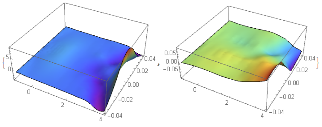
It is not unique solution, since we can apply some boundary condition for any border as well.



NDSolveValueshould solve your problem $\endgroup${x10,x20}inside region or on the border? $\endgroup$Plot3D[h1[x1, x2], {x1, -1, 4}, {x2, -0.04, 0.04}]you are plotting an unassigned function. You need to assigne the results of NDSolve to something (e.g. say,solutionfromNDSolve) then use something like:Plot3D[h1[x1, x2] /. solutionFromNDSolve, {x1, -1, 4}, {x2, -0.04, 0.04}]. $\endgroup$Gradientis an option forFindMinimum[]. Do you meanGrad[h1[x1, x2], {x1, x2}]==0andGrad[h2[x1, x2], {x1, x2}]==0? $\endgroup$