How to plot space of bistable solutions?

Question

I have the following ODE system

dx1 = -0.7 x1 y2 
dy1 = 0.7 x1 y2 + 1.7 (1-x1-y1) y2 - y1 
dx2 = -0.7 x2 y1 
dy2 = 0.7 x2 y1 + 1.7 (1-x2-y2) y1 - y2

I have found that, for initial conditions of the type $x_1=1-y_1, x_2=1-y_2$, solutions either:

• reach a steady-state where $y_1=y_2=0$
• or reach a steady-state where $y_1,y_2>0$.

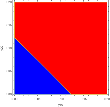
Now, I want to plot the plane of initial conditions $(y_1(0),y_2(0))$ and color each point in the plane blue or red depending on whether the steady-state falls in the first or second bucket.

I know how to use streamplot to explore the phase-space of solutions but I am not sure how to go about plotting the regions depending on the steady-state value. Any ideas would be much appreciated.

Answer 1

Here's an approach based on this answer by @ssch.

First, a function to solve the system and report the final values of y1[tmax] and y2[tmax]:

res[y10_?NumericQ, y20_?NumericQ] := Module[{sol},
  sol = NDSolve[{
    x1'[t] == -0.7 x1[t] y2[t],
    y1'[t] == 0.7 x1[t] y2[t] + 1.7 (1 - x1[t] - y1[t]) y2[t] - y1[t],
    x2'[t] == -0.7 x2[t] y1[t],
    y2'[t] == 0.7 x2[t] y1[t] + 1.7 (1 - x2[t] - y2[t]) y1[t] - y2[t],
    x1[0] == 1 - y10, y1[0] == y10, x2[0] == 1 - y20, y2[0] == y20},
    {x1, y1, x2, y2}, {t, 0, tmax}][[1]];
  Return[{y1[tmax], y2[tmax]} /. sol]
];

Then RegionPlot where the final values are close enough to {0, 0}:

tmax = 100;
tol = 10^-3;

RegionPlot[{Norm[res[y10, y20]] < tol, Norm[res[y10, y20]] > tol},
  {y10, 0, 0.2}, {y20, 0, 0.2}, 
  PlotPoints -> 20, MaxRecursion -> 2, PlotStyle -> {Blue, Red}, FrameLabel -> {y10, y20}]

See also this question.

Answer 2

Here's what I ended up doing in case anyone else has a similar question:

I used NDSolve to numerically solve the system. I then extracted the values of $y_1$ and $y_2$ at time $t=100$, which I know is sufficiently long for the system to reach steady-state. I then threshold the average of $y_1$ and $y_2$ and set the threshold close to zero. Then, I did this for multiple values of the initial conditions using Table and plotted the resulting array using arrayplot.

ArrayPlot[
 Table[(i1[100] + i2[100])/2 /. 
   NDSolve[{s1'[t] == -0.7 s1[t] i2[t], 
      i1'[t] ==  0.7 s1[t] i2[t] + 1.7 (1 - s1[t] - i1[t]) i2[t] - i1[t], 
      s2'[t] == -0.7 s2[t] i1[t], 
      i2'[t] == 0.7 s2[t] i1[t] + 1.7 (1 - s2[t] - i2[t]) i1[t] - i2[t], 
      i1[0] == p1, i2[0] == p2, s1[0] == 1 - p1, s2[0] == 1 - p2},
      {i1, i2}, {t, 0, 100}][[1]], {p1, 0, 1, 0.005}, {p2, 0, 1, 0.005}], 
   ColorFunction -> (If[# > 0.02, Red, Blue] &), DataReversed -> True]