We can plot the components of u by using ContourPlot3D like this
A = 1; r = 1; d = r^2 + x^2 + y^2 + z^2;
ContourPlot3D[{(2 A/d^2)*(x*z - r*y), (2 A/d^2) (r*x + y*z), (A/
     d^2)*(r^2 - x^2 - y^2 + z^2)}, {x, -3, 3}, {y, -3, 3}, {z, -3,
  3}]
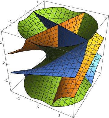
For the above plot, I took random values for $A$ and $r$.
Since your system of differential equation is coupled and nonlinear, so, I will straight away go for NDSolve.
d = r^2 + x[t]^2 + y[t]^2 + z[t]^2;
ux = (2*A/d^2)*(x[t]*z[t] - r*y[t]);
uy = (2*A/d^2)*(r*x[t] + y[t]*z[t]);
uz = 1/2*(A/d^2)*(r^2 - x[t]^2 - y[t]^2 + z[t]^2);
u = Sqrt[ux^2 + uy^2 + uz^2];
soln = NDSolve[{x'[t] == ux/Abs[u], y'[t] == uy/Abs[u],
    z'[t] == uz/Abs[u], x[0] == 0, y[0] == 1, z[0] == 0}, {x, y,
    z}, {t, 0, 50}];
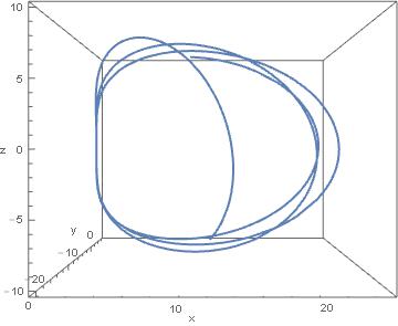
Finally ploting the results as a 3D,
ParametricPlot3D[{x[t], y[t], z[t]} /. soln, {t, 0, 50},
 PlotRange -> All, MaxRecursion -> 8, AxesLabel -> {"x", "y", "z"}, ViewPoint -> Front]
Edit
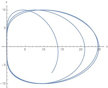
In responce to your xz-plane view comment, @J.M. suggested ParametericPlot,
ParametricPlot[{x[t], z[t]} /. soln, {t, 0, 250}, PlotRange -> All,
 MaxRecursion -> 8, AxesLabel -> {"x", "z"}]
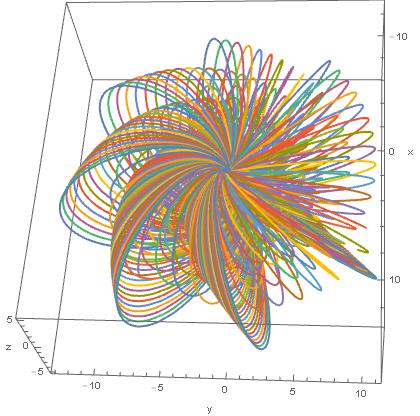
For set of different initial conditions, you can do something like this,
sol[x0_?NumericQ, y0_?NumericQ, z0_?NumericQ] :=NDSolve[{x'[t] == ux/Abs[u], y'[t] == uy/Abs[u], z'[t] == uz/Abs[u],
         x[0] == x0, y[0] == y0, z[0] == z0}, {x, y, z}, {t, 0, 250}];
    ParametricPlot3D[
     Evaluate[{x[t], y[t], z[t]} /. sol[#, #, #] & /@
       Range[2, 5, .1]], {t, 0, 250}, PlotRange -> All, MaxRecursion -> 8,
      AxesLabel -> {"x", "y", "z"}]


uon the right hand sides of the differential equations? $\endgroup$x'[t]=u_x/Abs[u_x]? Your system of differential equations is coupled nonlinear one, thus, we need specific numerical values forx0, y0andz0to be able to find a numerical solution. $\endgroup$