How to specify derivative boundary conditions for the gradient to be normal to the boundary?

Question

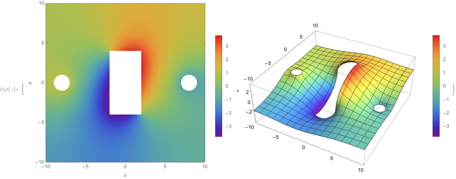
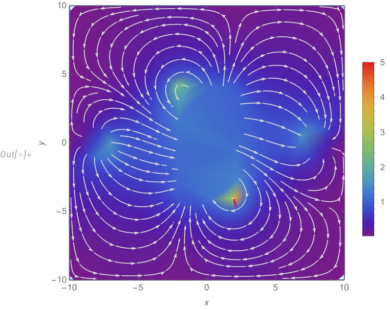
I'm currently modeling an electric field with 2 charges. To do so, I use NDSolveValue to solve a Laplacian with 2 Dirichlet conditions on the voltages of the charges, with which I am successfully able to do. However, I now try to add a rectangular conductor with free charges between them, and that's where I encounter my issue.

To set up a conductor, I subtract an additional object from the region and set up conditions on its borders such that the gradient of the field is always perpendicular to the boundary, (as electric field lines going in and out of the conductor are perpendicular to its surface) i.e. for top and bottom $u_x(x,y) = 0$, and for right and left $u_y(x,y)=0$. I tried using NeumannValue as in code below, but I encounter an error saying

"NDSolveValue::fembcdepderiv: Derivatives of dependent variables in boundary conditions are not supported with the Finite Element Method in this version of NDSolve."

I've looked through similar problems (link link, link), but the solutions proposed either didn't apply to this problem or didn't work for me.

My question is, how can I set up the Neumann boundary condition for the normal derivative to be equal to the gradient, so that the electric field goes perpendicularly inside the conductor? Alternatively, an existing function a-la Acoustic PDE would also work.

Needs["NDSolve`FEM`"];
(*Define Boundaries*)
boundaries = {{-10, -10}, {10, 10}};

air = Rectangle @@ boundaries;
object1 = Disk[{-8, 0}, 1];
object2 = Disk[{8, 0}, 1];
conductor = Rectangle[{-2, -4}, {2, 4}];
reg12 = RegionUnion[object1, object2, conductor];
reg = RegionDifference[air, reg12];

mesh = ToElementMesh[reg, Transpose[boundaries], 
   MeshRefinementFunction -> 
    Function[{vertices, area}, 
     area > 0.001 (0.1 + 10 Norm[Mean[vertices]])]];
mesh["Wireframe"]

eq = Laplacian[u[x, y], {x, y}]; V1 = 1; V2 = -1;
bc = {DirichletCondition[u[x, y] == V1, 
    Region`RegionProperty[RegionBoundary[object1], {x, y}, 
       "FastDescription"][[1]][[2]]], 
   DirichletCondition[u[x, y] == V2, 
    Region`RegionProperty[RegionBoundary[object2], {x, y}, 
       "FastDescription"][[1]][[2]]]};
U = NDSolveValue[
   {eq == 
     NeumannValue[
       Derivative[1, 0][u][x, 
        y], (-4 <= y <= 4 && (x == 2 || 2 + x == 0))]
      + NeumannValue[
       Derivative[0, 1][u][x, 
        y], (-2 <= x <= 2 && (y == 4 || 4 + y == 0))],
    bc},
   u, {x, y} \[Element] mesh];

ef = -Grad[U[x, y], {x, y}];

Visualization code if you manage to make it work:

{
 DensityPlot[U[x, y], {x, y} \[Element] reg,
  ColorFunction -> "Rainbow", PlotLegends -> Automatic, 
  FrameLabel -> Automatic, PlotPoints -> 50, 
  PlotRange -> Transpose[boundaries], ImageSize -> Medium],
 Plot3D[U[x, y], {x, y} \[Element] reg,
  ColorFunction -> "Rainbow", PlotLegends -> Automatic, 
  PlotPoints -> 50, PlotRange -> Transpose[boundaries], 
  ImageSize -> Medium]
 }

StreamDensityPlot[Evaluate[ef], {x, y} \[Element] reg, 
 ColorFunction -> "Rainbow", PlotLegends -> Automatic, 
 FrameLabel -> {x, y}, StreamColorFunction -> None, 
 StreamStyle -> LightGray, PlotRange -> Transpose[boundaries], 
 ImageSize -> Medium]

Answer 1

Is this what you are looking for:

U = NDSolveValue[{eq == 
     NeumannValue[
       Indexed[BoundaryUnitNormal[x, y], 
        1], (-4 <= y <= 4 && (x == 2 || 2 + x == 0))] + 
      NeumannValue[
       Indexed[BoundaryUnitNormal[x, y], 
        2], (-2 <= x <= 2 && (y == 4 || 4 + y == 0))], bc}, 
   u, {x, y} \[Element] mesh];

ef = -Grad[U[x, y], {x, y}];