The condition x[t] == 0 && p[t] > 0 is not true very often, if at all, for the initial conditions tried in the OP's differential equation. It would not explain why your session would encounter a such a problem. (I haven't gotten such an error in a very long time. I always associated it with a bug. It was often unreproducible. If you can reliably reproduce your problem, then you should file a report with Wolfram Research.)
Perhaps the problem is associated with the fact that abcdata turns out not be three data sets of points. For me, ListPlot detects an error and report it, which is what should happen for you. The source of the problem is that your code does not handle the case that no points are sown and the part {1, -1} in Reap[NDSolve[<>]][[1,-1]] does not exist. I get an error message to that effect, and you should have, too. If you don't get that error, then the crash is occurring during the Reap/NDSolve.
That's what I can say about the Mathematica problem. There also seems to be some problem with the mathematical setup. The section chosen for the Poincaré map is the half of the hyperplane x == 0 for which p > 0. Unfortunately this does not appear to be transverse to the flow, nor do the orbits return to it.
The following can give a picture of why this section will not work. I'll save the solution return by NDSolve in nd, which I use for plotting.
Clear[psect]

abc = {x'[t] == p[t], p'[t] == -x[t] - y[t], y'[t] == q[t], q'[t] == -y[t] - x[t]};

psect[{x0_, p0_, y0_, q0_}] :=
 Reap[nd[{x0, p0, y0, q0}] =
    NDSolve[{abc, x[0] == x0, p[0] == p0, y[0] == y0, q[0] == q0,
      WhenEvent[x[t] == 0 && p[t] > 0, Sow[{y[t], q[t]}]]},
      {x[t], p[t], y[t], q[t]}, {t, 0, 1000}, MaxSteps -> ∞]
  ][[-1, 1]]

ivdata = {{1, 1, 1, 2}, {2, 1, -1, 2}, {3, 2, -1, 1}};

abcdata = Map[psect, ivdata];
Part::partw: Part 1 of {} does not exist. >>
...
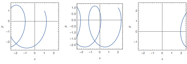
We can see here that the hyperplane section is crossed 0, 1, 0 times respectively from the three initial starting points ivdata:
GraphicsRow[
 ParametricPlot[{x[t], p[t]} /. nd[#], {t, 0, 1000},
    MaxRecursion -> 10,
    AspectRatio -> 1, Frame -> True, FrameLabel -> {x, p},
    AxesOrigin -> {0, 0}, PlotRange -> {{-2.5, 2.5}, All}] & /@ ivdata
 ]

The system is linear with constant coefficients. We can see that the value of x[t] has a linear term in t that can explain the steady looping movement of the solution along the x axis.
ds[{x0_, p0_, y0_, q0_}] :=
 DSolve[{abc, x[0] == x0, p[0] == p0, y[0] == y0, q[0] == q0},
  {x[t], p[t], y[t], q[t]}, t]

Simplify[ExpToTrig[x[t] /. ds /@ ivdata]]
(*
  {{Cos[Sqrt[2] t] + 1/4 (-2 t + 3 Sqrt[2] Sin[Sqrt[2] t])},
   {1/4 (6 - 2 t + 2 Cos[Sqrt[2] t] + 3 Sqrt[2] Sin[Sqrt[2] t])},
   {Cos[Sqrt[2] t] + 1/4 (8 + 2 t + 3 Sqrt[2] Sin[Sqrt[2] t])}}
*)
There are periodic solutions (if p0 = q0 = 0),

