Short answer
Yes, we can. With good CPU and memory resources even in a very high quality.
Introduction
I stumbled over this issue while thinking about this answer here where in my opinion a high quality vectorizer would be of great help. Then I read about how this is done in real applications and read the documentation to Potrace which is the underlying tracer of Inkscape.
At this point it was clear to me, that we can achieve this with the tools included into Mathematica. The only question was, whether it gives reasonable results.
In the following sections I explain what steps are necessary to vectorize a color image in Mathematica.
Implementation
Segmentation
The first thing one has to understand is that color vectorization happens in multiple scans, which means regions of equal color will be transformed in a polygon-representation. A usual 8 bit color image with 256^3 possible colors has in the worst case a different color for each pixel.
In a vectorized image you want not only a realistic look but if possible only a few large regions to keep the number of polygons to a reasonable number. Therefore, what you have to do is to break you input image into regions with similar colors, with whatever definition of similar. Preferably, those regions should be not too small. This depends strongly on the input and cannot always be prevented.
Assume the following image

One fast and easy way to segment this image is to use ColorQuantize.
img = Import["https://i.sstatic.net/F5kJ2.png"];
quantized = ColorQuantize[img, 10, Dithering -> False]
You can specify the number of colors in the result (10 here) and later we will transform the regions of every color on after another into a vector graphic. The option Dithering->False is important here, otherwise the algorithm would try to minimize the quantization error by dithering which would lead to very small regions.
We could now look on the colors in the output image and would see that there are exactly 10 different rgb-values
cols = Union[Flatten[ImageData[quantized, "Byte"], 1]]

(* {{19, 24, 18}, {27, 36, 23}, {40, 47, 28}, {43, 49, 30}, {50,75, 37},
   {84, 79, 58}, {101, 139, 121}, {160, 95, 43}, {176, 153, 96}, {177, 183, 167}}
*)
We will use these colors later when we draw the polygons. Let's store them
colors = RGBColor @@ (#/255.) & /@ cols;
Separating the regions
Now we want to extract all different color regions. We need a binary mask for every region. We can create this by extracting the image data and then setting all pixel to zero which are not the specified color. If we do this for all colors we get 10 different binary masks
data = ImageData[quantized, "Byte", DataReversed -> True];
masks = Block[{data =
       Image[data /. {Except[cols[[#]], {_Integer ..}] :> 0,
          cols[[#]] :> 1}]},
     Developer`ToPackedArray[
      ImageData[GaussianFilter[Opening[data, 0], 1], "Real"]]] & /@
   Range[Length[cols]];

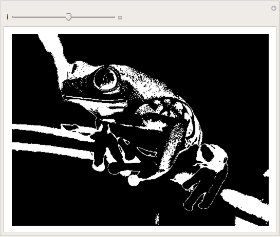
Manipulate[
 Image[Reverse[masks[[i]]]],
 {i, 1, Length[cols], 1}]

There are two extra function I used which can be adjusted to further smooth the input image or to remove very small objects: GaussianFilter and Opening
Vectorizing
The binary masks we created representing nothing more then the regions which should later have a special color in the final image. To plot those regions we can use RegionPlot if we interpolating functions from the matrices and then defining a region to have a value greater then 1/2.
The following RegionPlot take the number of a specific region, uses its color and interpolating function and draws a high quality polygon-graphic:
ipfuncs = ListInterpolation /@ masks;
{nx, ny} = ImageDimensions[img]
With[{c = colors[[#]]},
   RegionPlot[ipfuncs[[#]][y, x] > 0.4, {x, 1, nx}, {y, 1, ny},
    PlotStyle -> c, BoundaryStyle -> None, Frame -> False,
    AspectRatio -> Automatic, PlotPoints -> 200, MaxRecursion -> 2,
    PlotRange -> {{1, nx}, {1, ny}}]] &[6]

The final step is, to do this for all regions and combine all Graphics by a Show. Let's pack this all in a function
Options[TraceBitmap] = {
   TraceLevels -> 2,
   Smooth -> 1,
   RemoveSpeckles -> 1,
   PlotPoints -> 50,
   MaxRecursion -> 3
   };
TraceBitmap[img_Image, opts : OptionsPattern[]] :=
 Module[{data, nx, ny, levels, smoothing, speckles, imageColors,
   rgbValues, levelMasks},

  {levels, smoothing, speckles} =
   OptionValue[{TraceLevels, Smooth, RemoveSpeckles}];
  {nx, ny} = ImageDimensions[img];
  data = ImageData[ColorQuantize[img, levels, Dithering -> False],
    "Byte", DataReversed -> True];
  imageColors = Union[Flatten[data, 1]];
  rgbValues = RGBColor @@ (#/255.) & /@ imageColors;
  levelMasks =
   Block[{bm =
        Image[data /. {Except[imageColors[[#]], {_Integer ..}] :> 0,
           imageColors[[#]] :> 1}]},
      ListInterpolation@
       Developer`ToPackedArray[
        ImageData[GaussianFilter[Opening[bm, speckles], smoothing],
         "Real"]]] & /@ Range[levels];

  Show[RegionPlot[levelMasks[[#]][y, x] > .4, {x, 1, nx}, {y, 1, ny},
      PlotStyle -> rgbValues[[#]],
      BoundaryStyle -> Directive[rgbValues[[#]]], Frame -> False,
      AspectRatio -> Automatic, PlotRange -> {{1, nx}, {1, ny}},
      PlotPoints -> OptionValue[PlotPoints],
      MaxRecursion -> OptionValue[MaxRecursion]] & /@ Range[levels]
   ]
  ]
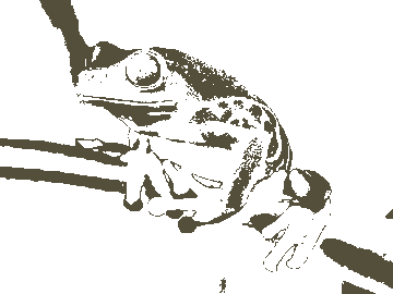
Results
TraceBitmap[img, TraceLevels -> 20, MaxRecursion -> 3,
 PlotPoints -> 100, RemoveSpeckles -> 0]

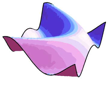
And, of course..
img = Rasterize[
   Plot3D[Sin[x + y^2], {x, -3, 3}, {y, -2, 2}, Boxed -> False,
    Axes -> False, Mesh -> None, BoundaryStyle -> Thickness[.01]],
   "Image", ImageSize -> 500];
TraceBitmap[img, TraceLevels -> 20, MaxRecursion -> 3,
 PlotPoints -> 100, RemoveSpeckles -> 0]
