ListDensityPlot using a customized colorfunction

Question

I would like to plot a figure using colorfunction in Mathematica. I opened the "Color Schemes" from the Palettes menu, but did not find a proper colorfunction.

Questions: Please see the below image.

1. Can I use only a part of "Rainbow" colorfunction? I do not want to use the dark blue side. For this case, how to rescale the new color range to be 0-1?
2. Furthermore, it looks the red side of "Rainbow" is not dark enough. Can I further add a red part of "Visible Spectrum" on it? and then rescale the new color range to be 0-1 again.

May someone help me? Thank you in advance.

Answer 1

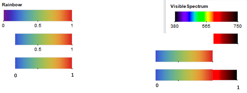
We start by defining a function for visualizing color functions:

colorbar[cf_] := DensityPlot[
  x,
  {x, 0, 370},
  {y, 0, 50},
  ColorFunction -> cf,
  ColorFunctionScaling -> True,
  AspectRatio -> Automatic,
  PlotRangePadding -> 10,
  FrameTicks -> {
    {None, None},
    {
     Transpose[{
       Subdivide[370, 5],
       N@Subdivide[5]
       }],
     None}
    }]

The problems that you mention can be solved using Rescale.

Using only a part of the rainbow color scheme:

cf = ColorData["Rainbow", Rescale[#, {0, 1}, {0.25, 1}]] &;
colorbar[cf]

Using only a part of the visible spectrum color function:

cf = ColorData["VisibleSpectrum", Rescale[#, {0, 1}, {625, 750}]] &;
colorbar[cf]

Combining parts from different color functions:

cf = Which[
    # < 0.8,
    ColorData["Rainbow", Rescale[#, {0, 0.8}, {0.25, 1}]],
    # >= 0.8,
    ColorData["VisibleSpectrum", Rescale[#, {0.8, 1}, {625, 750}]]
    ] &;
colorbar[cf]

Another way is to sample colors from the color functions and put them together using Blend:

cf = Blend[Join[
     Table[
      {0.8 (x - 0.25)/(1 - 0.25), ColorData["Rainbow", x]},
      {x, 0.25, 1, 0.01}],
     Table[
      {0.8 + 0.2 (x - 625)/(750 - 625), ColorData["VisibleSpectrum", x]},
      {x, 625, 750}
      ]
     ], #] &;
colorbar[cf]