How to mimic MATLAB parula color scheme efficiently? [duplicate]

Question

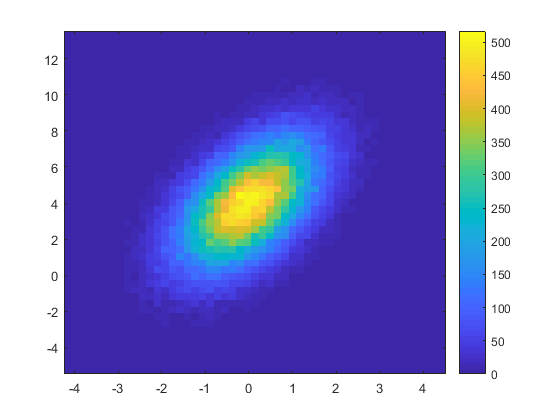
Does anybody know how to mimic MATLAB's default scheme for DensityPlot, just like this picture shows:

---

update

There are several answers already, Thank you very much.

But I am still wondering how to make the colorscheme more efficient.

Compare below cases:

<< "http://pastebin.com/raw/sqYFdrkY";
dd = Partition[Flatten[Table[Sin[x] Sin[y], {x, -4, 4, 0.01}, {y, -3, 3, 0.2}]], 2];
gnuplotTraditional = RGBColor[Sqrt[#], #^3, Sin[2 π #]] &;

ListDensityPlot[dd, PlotRange -> All, 
   ColorFunction -> ParulaCM]; // AbsoluteTiming
ListDensityPlot[dd, PlotRange -> All, 
   ColorFunction -> ColorData["SunsetColors"]]; // AbsoluteTiming
ListDensityPlot[dd, PlotRange -> All, 
   ColorFunction -> gnuplotTraditional]; // AbsoluteTiming

The timing result on my computer is

{1.25649, Null}

{0.496294, Null}

{0.584826, Null}

So methods using Blend on color list is way too slow (consider ListDensityPlot is already very slow in Mathematica with large data).

So is there a succinct color formula for MATLAB's parula?

Answer 1

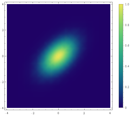
I suggest you take a look at all available color shemes.

The nearest one to your image seems to be "BlueGreenYellow"

So:

DensityPlot[Exp[-(x^2 + y^2) + y*x], {x, -4, 4}, {y, -4, 4}, 
 PlotLegends -> Automatic, ColorFunction -> "BlueGreenYellow", 
 PlotRange -> All]

Though, we can agree, this is not equal. We therefore can extract the matlab color sheme from your image:

{w, h} = ImageDimensions[matlabImage];
colorBar = ImageTake[matlabImage, All, {w - 95, w - 94}];
colorBarData = 
  RGBColor /@ 
   Select[Flatten[ImageData[colorBar], 1], 
    Total[#] != 3 && Total[#] != 0 &];
colorBarData = colorBarData[[3 ;; -3]];
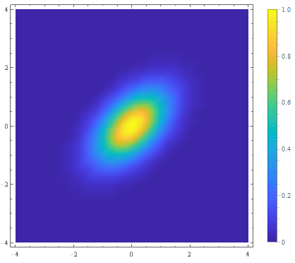
matlabColorFunction[x_] := Blend[Reverse@colorBarData, x];

Where matalbImage is the image yoU've posted. We can use this therefore with

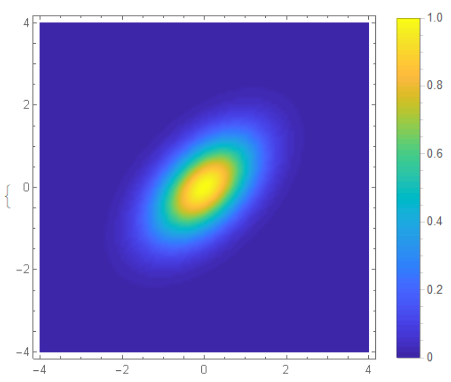
DensityPlot[Exp[-(x^2 + y^2) + y*x], {x, -4, 4}, {y, -4, 4}, 
 PlotLegends -> Automatic, ColorFunction -> matlabColorFunction, 
 ColorFunctionScaling -> True, PlotRange -> All]

Which looks really equal to what you have given there.

Answer 2

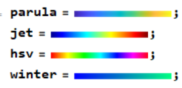
We can use color data from legend. Go to https://www.mathworks.com/help/matlab/ref/colormap.html and copy the legend and put it in Mathematica

colorName = {parula, jet, hsv, winter};

{col, row} = ImageDimensions /@ colorName // First;

ParulaMMA = 
  Module[{colorlist}, 
   colorlist = 
    Catenate@
     ImageData@ImageTake[parula, {Round[row/2], Round[row/2]}, All];
   Evaluate[Blend[RGBColor @@@ colorlist, #] &]];

JetMMA = Module[{colorlist}, 
   colorlist = 
    Catenate@
     ImageData@ImageTake[jet, {Round[row/2], Round[row/2]}, All];
   Evaluate[Blend[RGBColor @@@ colorlist, #] &]];

HsvMMA = Module[{colorlist}, 
   colorlist = 
    Catenate@
     ImageData@ImageTake[hsv, {Round[row/2], Round[row/2]}, All];
   Evaluate[Blend[RGBColor @@@ colorlist, #] &]];

WinterMMA = 
  Module[{colorlist}, 
   colorlist = 
    Catenate@
     ImageData@ImageTake[winter, {Round[row/2], Round[row/2]}, All];
   Evaluate[Blend[RGBColor @@@ colorlist, #] &]];   


 Legended[DensityPlot[Exp[-(x^2 + y^2) + y*x], {x, -4, 4}, {y, -4, 4}, 
    PlotRange -> All, ColorFunction -> #, PlotPoints -> 100, 
    ImageSize -> 220], BarLegend[{#, {0, 1}}]] & /@ {ParulaMMA, 
  JetMMA, HsvMMA, WinterMMA}