8
$\begingroup$

I am making a 2D scatter plot with some data, let us say:

data = RandomReal[{0, 10}, {22, 2}];
samplecode = Table["sample " <> ToString[i], {i, 1, Dimensions[data][[1]]}];
ListPlot[data,
  Frame -> True, 
  Axes -> None, 
  PlotRange -> All,
  PlotStyle -> {AbsolutePointSize[8], Red}, 
  BaseStyle -> {FontSize -> 32, FontFamily -> "Arial"},
  FrameStyle -> Directive[Black, AbsoluteThickness[3]], 
  GridLines -> {None, {0}}, 
  Epilog -> 
    {Red, 
     MapThread[
       Text[Style[#1, FontSize -> 12], #2, {0.5, -1.5}] &, 
       {samplecode,data}]},
   AspectRatio -> 1]

The plot looks very busy and, sometimes, the labels that I am adding via Epilog end up overlapping with each other.

What I would like to do is improve readability by

  • putting the labels on the right hand side of the plot (outside or inside the plot area does not matter) and connect them to the point they belong to with an arrow

  • color coding each point, arrow and label set

I can do this by hand but, this takes a long time when the number of points is high (normally 50 or so). How can I implement this progamatically?

$\endgroup$
5
  • $\begingroup$ In V11 there is a Callout though I am not sure how far one can go with it. $\endgroup$
    – Kuba
    Nov 28, 2016 at 12:46
  • $\begingroup$ I am looking for a solution applicable in V10.0.2 (my system) $\endgroup$
    – Luigi
    Nov 28, 2016 at 13:41
  • $\begingroup$ Related: (13906) and (126855). $\endgroup$
    – corey979
    Nov 28, 2016 at 17:59
  • $\begingroup$ Related to the Map-Labeling problem en.wikipedia.org/wiki/Automatic_label_placement -- Maybe some wizard can hack GeoLabels... $\endgroup$
    – A.G.
    Nov 29, 2016 at 3:44
  • $\begingroup$ I have posted a whole new answer that provides a tool from making persistent movable labels. $\endgroup$
    – m_goldberg
    Dec 1, 2016 at 8:03

7 Answers 7

5
$\begingroup$

I deleted my earlier answer because I felt it just wasn't good enough. To be good enough for real-life use, the answer needs to make the labels persist over re-evaluations of the plot and over Mathematica sessions.

Here is a solution that I feel better about.

Code

With[{
  canNotSave1 = 
    (Row[
       {Style[
         "Can not save text specifications. Current text positions are: ", 
         "SR"],
       #}] &),
  canNotSave2 =
    Row[
      {Style["First argument to ", "SR"], "TexTool", 
       Style[" must be a string for pesistence to be enabled", "SR"]}]},
  textTool[
      itemSource : (_String | {_Text ..}),
      plotSource : (_Graphics | _GraphicsComplex)] :=
    DynamicModule[{items, nItems, plot, buttons, pt, indx},
      items =
        Switch[itemSource,
         _String, LocalSymbol[itemSource],
        {_Text ..}, itemSource];
      nItems = Length[items];
      Do[pt[i] = items[[i, 2]], {i, nItems}];
      Panel[
        Column[
          {Style["Text Positioning Tool", "SB", 16],
           EventHandler[
             Dynamic @ Panel[plot, Background -> White],
             {"MouseDown" :>
                (indx =
                   First @
                     Nearest[
                       Table[pt[i] -> i, {i, nItems}],
                       MousePosition["Graphics"]]; 
                 pt[indx] = MousePosition["Graphics"]),
              "MouseDragged" :>
                (pt[indx] = MousePosition["Graphics"])}],
           Item[Dynamic @ buttons, Alignment -> Right]}]],
      Initialization :> (
        plot :=
          Module[{lbls = items},
            Do[lbls[[i, 2]] = pt[i], {i, nItems}];
            Show[plotSource, Graphics[lbls]]];
        buttons :=
          Row[
            {Button["Print", Print[plot], Method -> "Queued"],
             Button["Revert", Do[pt[i] = items[[i, 2]], {i, nItems}]],
             Button["Save",
               Switch[itemSource,
                _String, 
                  Do[items[[i, 2]] = pt[i], {i, nItems}];
                  LocalSymbol[itemSource] = items,
                {_Text ..},
                  Print[
                    Column[
                      {canNotSave1[pt /@ Range[nItems]], 
                       canNotSave2}]]]]}])]]

Usage

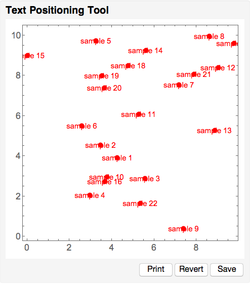
textTool enables you to do the following things with plots:

  • Interactively move text items in a panel displaying the plot and the text.

  • Edit the plot code and re-evaluate it without disturbing the positioning work already done on the text (textTool never modifies the plot you are working on).

  • Save the specification of the text items and their locations so you can take up work from where you left off after re-evaluating the plot or in a future Mathematica session.

  • Make snapshots of your work as you go. Each of these is printed in a new cell.

textTool requires two arguments.

  • First argument

    The name of a local symbol (see LocalSymbol) where the text item specifications will be stored. In this case persistence is enabled. Arrangements of the text items will persist over re-evaluation of textTool in current session or in a future session.

    Or a list specifying the text items it is to display. The list takes the form {Text[...], Text[...], ..., Text[...]}. In this case persistence of the text items is disabled. Nonetheless, this can be useful in the early stages of text layout.

  • Second argument

    A graphics object which will form the background on which the text items will can be moved about.

User interface

  • Clicking to select a text item for dragging should be done near the center of the item. Otherwise, when two large items are close together, the one selected may not be the one intended. This can happen because the mouse cursor can be closer to center of one item even when it appears to be hovering over another.

  • textTool has three buttons.

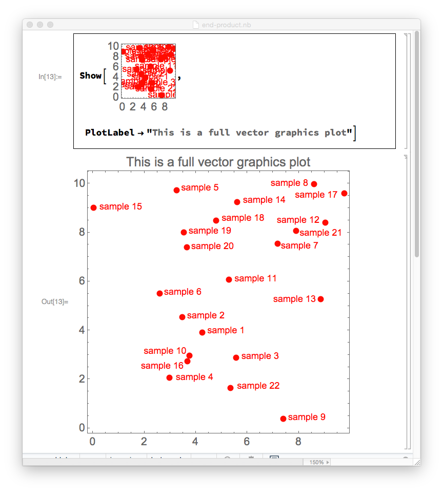
  • Clicking on the Print button prints the textTool workspace contents in a new cell. This is not a raster image, but a full-fledged plot. It is the the tool's end-product. This is what you insert (by cut and paste) into any notebook or CDF as the fully labeled plot. You can even use it as an input for further processing (see Screen capture below).

  • Clicking on the Revert button restores the textTool workspace to the way it was when you started it or to when you did your last save.

Notes

  • If you modify your plot, you must evaluate your textTool expression to work with the modified plot. If the first argument is the name of a local symbol, all previous label positioning work will be preserved. They will also be preserved across sessions.

  • textTool uses a local symbol to store your labels between textTool sessions or between Mathematica sessions. Clicking of the Save button both updates the local symbol and updates the positions that the Revert button will use.

  • The directory where the text item specifications are stored can be found by evaluating $LocalSymbolBase. The file containing the specifications is a normal text file.

  • When the first argument given to textTool is an actual list of text items rather than a local symbol name, persistence will be disabled. If the Save button is clicked on, a message will be printed warning of this and giving the current locations of the text items, so not all will be lost. If these positions are valuable, they can be inserted into the code that created the list of Text objects.

    An example of this:

msg

Test case

data = (SeedRandom[42]; RandomReal[{0, 10}, {22, 2}]);

Here is a text item specification of the first kind.

labels =
  With[
    {lbls =
       Table[
         Style["sample " <> ToString[i], 12, FontColor -> Red], 
         {i, 1, Length[data]}]},
    Thread[Text[lbls, data]]];

And this will convert it so you can use a specification of the second kind.

LocalSymbol["LabelsForScatterPlot"] = labels;

A plot to position the text items 0n.

scatterPlot =
  ListPlot[data,
    BaseStyle -> {FontSize -> 14, FontFamily -> "Arial"},
    Frame -> True,
    Axes -> None,
    PlotRange -> All,
    PlotStyle -> {AbsolutePointSize[8], Red},
    AspectRatio -> 1];

textTool["LabelsForScatterPlot", scatterPlot]

texttool

Editing the text items (updated)

Should you need to edit the text item specifications, you can recover them in editable form by evaluating

CellPrint[ExpressionCell[InputForm @ LocalSymbol["LabelsForScatterPlot"], "Input"]]

spec

After editing, it should look something like the following (I show one item label having been changed to have black text). Evaluate this cell to update your text item specifications.

edit

Screen capture

A plot printed from textTool being used as input to Show.

screen-shot

$\endgroup$
2
  • $\begingroup$ thanks this is really a great solution to my issue. works well , quick and simple to use. Cheers $\endgroup$
    – Luigi
    Dec 2, 2016 at 8:21
  • $\begingroup$ @Luigi. I have fixed a bug in the code for recovering the text item specifications, so the created code cell is ready for editing without having to fool with the Cell menu. See my update to that section above. $\endgroup$
    – m_goldberg
    Dec 3, 2016 at 13:10
5
$\begingroup$

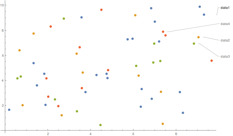
This answer uses PlotLabels introduced in version 10.4. It has the merit of being a literal answer to the question asked in case someone else finds it useful.

PlotLabels automatically places a label for each dataset plotted.

data1 = RandomReal[{0, 10}, {11, 2}];
data2 = RandomReal[{0, 10}, {11, 2}];
data3 = RandomReal[{0, 10}, {11, 2}];
data4 = RandomReal[{0, 10}, {11, 2}];
ListPlot[{data, data2, data3, data4}, 
 PlotLabels -> {"data1", "data2", "data3", "data4"}]

datasets

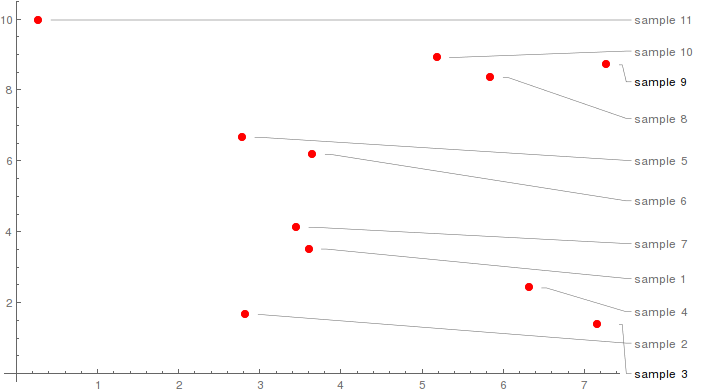
It follows that an easy way to programmatically assign a label to each datapoint is to make each point a dataset. You can then assign a color for the whole scatter plot.

data = RandomReal[{0, 10}, {11, 2}];
ListPlot[Partition[data, 1], 
 PlotLabels -> Table["sample " <> ToString[i], {i, 1, 11}], 
 PlotStyle -> Red]

datapoints

This solution can still lead to a crowded margin, but it's very simple to implement. Also consider using Callout as indicated by @Kuba.

$\endgroup$
3
$\begingroup$

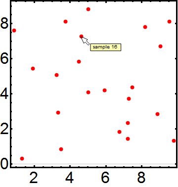
If you are using this in an active notebook (i.e, not trying to produce a static plot that you want to output and share) you might think about using Tooltip.

Tooltip is absent from the screen but will appear when you hover the mouse close to a particular point.

ListPlot[
 Table[
  Tooltip[data[[i]], "sample " <> ToString[i]],
   {i, Length@data}
  ],
 Frame -> True,
 Axes -> None,
 PlotRange -> All,
 PlotStyle -> {AbsolutePointSize[8], Red},
 BaseStyle -> {FontSize -> 32, FontFamily -> "Arial"},
 FrameStyle -> Directive[Black, AbsoluteThickness[3]],
 GridLines -> {None, {0}},
 AspectRatio -> 1
 ]

Mathematica graphics

$\endgroup$
1
  • $\begingroup$ thanks. I am actually trying to make a 'static' plot to be exported and shared. So I will not be able to use Tooltip. $\endgroup$
    – Luigi
    Nov 29, 2016 at 10:04
2
$\begingroup$

I have written a function entitled "arrowedLetteredImage" simplifying drawing arrows on a technical sketches. Please find below (1) its description, (2) the function itself, and, finally, (3) an example of application to your specific case:

(1). Description:

The function arrowedLetteredImage[pict, letter, imageSize] is designed in order to help to place an arrow with a letter at its end onto an preexisting image. The arguments: image is an image or a graphics object. letter is any string. imageSize is an integer giving the size of the overall image. The sliders are self-explaining The resulting image is assigned to a global variable entitled "image" upon pressing of the button. It returns the desired image upon evaluation in any other cell.

(2) The function arrowedLetteredImage

    arrowedLetteredImage[pict_, letter_String, imageSize_Integer] := 
 DynamicModule[{ptA, ptB, xA, yA, thicknessA = 0.015, 
   arrowHeadA = 0.07, arrowColorA = Red, letterColorA = Black, 
   letterSizeA = 12, letterFaceA = Plain, 
   im = Image[pict, ImageSize -> imageSize]},
  Column[{
    Manipulate[
     ptA = pt1;
     ptB = pt2;
     xA = x;
     yA = y;
     thicknessA = arrowThickness;
     arrowHeadA = arrowHead;
     arrowColorA = arrowColor;
     letterColorA = letterColor;
     letterSizeA = letterSize;
     letterFaceA = letterFace;
     Show[{
       im,
       Graphics[{arrowColor, Thickness[arrowThickness], 
         Arrowheads[arrowHead], Arrow[{pt1, pt2}]}],
       Graphics[
        Text[Style[letter, letterColor, letterSize, letterFace], 
         pt1 + {x, y}]],
       Graphics[{Locator[pt1], Locator[pt2]}]
       }], 
     Column[{
       Row[{
         Control[{{pt1, IntegerPart[ImageDimensions[im]*2/3]}}], 
         Control[{{pt2, IntegerPart[ImageDimensions[im]*1/3]}}]
         }],
       Row[{
         Column[{

           Control[{{x, 
              ImageDimensions[im][[1]]/20}, -ImageDimensions[im][[1]]/
              4, ImageDimensions[im][[1]]/4}],

           Control[{{y, 
              ImageDimensions[im][[1]]/20}, -ImageDimensions[im][[1]]/
              4, ImageDimensions[im][[1]]/4}],
           Row[{

             Control[{{letterSize, 12}, {10, 11, 12, 13, 14, 15, 14, 
                15, 16, 18, 20, 24, 28, 30}}], 
             Control[{{letterFace, Plain}, {Plain, Italic, Bold}}]
             }],
           Control[{letterColor, Black}]

           }], Spacer[10],

         Column[{
           Control[{{arrowThickness, 0.015}, 0.001, 0.03}],
           Control[{{arrowHead, 0.07}, 0.001, 0.2}],
           Control[{arrowColor, Red}]

           }]
         }]
       }], 
     ControlType -> {Locator, Locator, Slider, Slider, PopupMenu, 
       PopupMenu, ColorSlider, Slider, Slider, ColorSlider}, 
     SaveDefinitions -> True
     ],

    Button["Get the image", Clear[image]; image = Show[{
        im,
        Graphics[{arrowColorA, Thickness[thicknessA], 
          Arrowheads[arrowHeadA], Arrow[{ptA, ptB}]}],
        Graphics[
         Text[Style[letter, letterColorA, letterSizeA, letterFaceA], 
          ptA + {xA, yA}]]
        }]]
    }]]

(3) Example of operation.

Let us first take your plot, but slightly change the data, such that each point represents a nested list itself:

 data = RandomReal[{0, 10}, {10, 2}] /. {x_, y_} -> {{x, y}}

(* {{{1.13488, 0.816025}}, {{0.316584, 8.15396}}, {{4.24867, 
   7.87471}}, {{7.77772, 9.58762}}, {{8.37356, 5.40324}}, {{2.83593, 
   6.38637}}, {{1.08502, 5.80997}}, {{8.54839, 4.12735}}, {{8.21854, 
   1.60547}}, {{6.85684, 0.214468}}} *)

I took only 10 points to clarify the demonstration. In such a case we can apply markers to the plot:

pl = ListPlot[data, Frame -> True, Axes -> None, PlotRange -> All, 
  PlotStyle -> {AbsolutePointSize[8], Red}, 
  BaseStyle -> {FontSize -> 32, FontFamily -> "Arial"}, 
  FrameStyle -> Directive[Black, AbsoluteThickness[3]], 
  GridLines -> {None, {0}}, AspectRatio -> 1, 
  PlotMarkers -> Automatic]
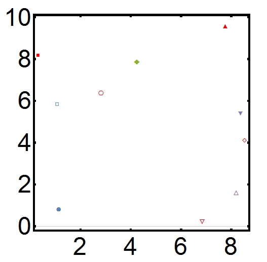
enter image description here

Now let us wrap the plot pl by the arrowedLetteredImage function

arrowedLetteredImage[pl, "Smpl 1", 300]

and evaluate it.
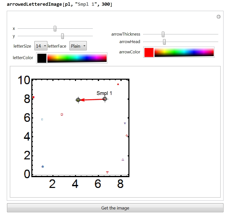
enter image description here

Using the locators position the arrow, using the sliders on your right choose the size of the arrow shaft and head. Using the color slider choose the arrow color. Using the sliders on your left choose the annotation position, and with the popup menu choose its font size and face. Done. Now press the button "Get the image" below the panel and evaluate the variable "image" in a separate cell.

image
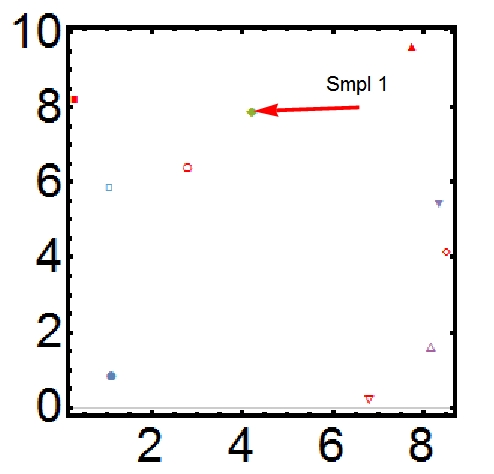
enter image description here

Done. You may repeat this few times to position as many arrows as you need.

Have fun!

$\endgroup$
1
  • $\begingroup$ this is a great routine! However, if I have to do it for 20-30 points on a graph, I would rather have it automated. Thanks for sharing. $\endgroup$
    – Luigi
    Nov 29, 2016 at 10:28
1
$\begingroup$

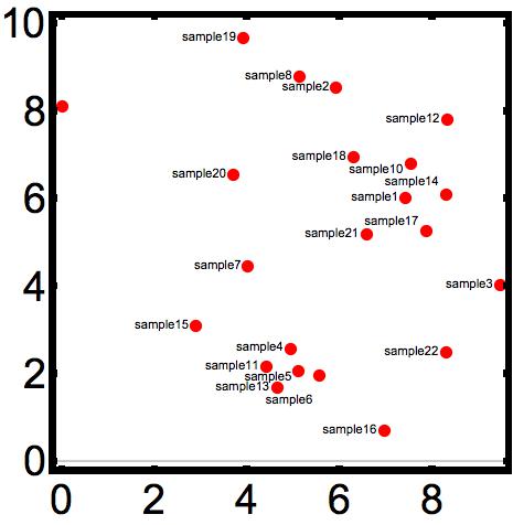
I think this has been nicely answered by @m_goldberg and @musang. When I have encountered this problem, I was never happy with the results and so solved it with a little brute force. The basic idea is to define a jitter function that moves the labels up or down a bit. One can then fine tune the result as much as one wishes to get an aesthetically pleasing plot. This survives repeated evaluations (although not repeated RandomReal seeds!). Here is the function:

    jitterF[b_String] := Module[{ba},
  ba = <|
    "sample5" -> -.1,
    "sample4" -> -.15,
    "sample14" -> -1.5,
    "sample10" -> .9,
    "sample17" -> -1.,
    "sample6" -> 3.,
    "sample5" -> .9
    |>;
  If[NumberQ[ba[b]], ba[b], 0.]
  ]

To get the data in the input form, I use:

dataL = Flatten[#] & /@ ({samplecode, data}\[Transpose])

And then Show the plot and a Graphics construct containing the labels.

   Show[ListPlot[data, 
      Frame -> True, 
      Axes -> None, 
      PlotRange -> All, 
      PlotStyle -> {AbsolutePointSize[8], Red}, 
      BaseStyle -> {FontSize -> 32, FontFamily -> "Arial"}, 
      FrameStyle -> Directive[Black, AbsoluteThickness[3]], 
      GridLines -> {None, {0}}, AspectRatio -> 1], 
     Graphics[Map[
       Text[Style[First[#], Small, Black], Rest[#], {1.25,jitterF[First[#]]}]&, 
       dataL[[1 ;; Length[dataL]]]]]]

enter image description here

This can clearly be improved (note that one of labels is trimmed on the left), but converting the function to a jitterUpDown and adding jitterLeftRight would be pretty straightforward.

$\endgroup$
1
$\begingroup$

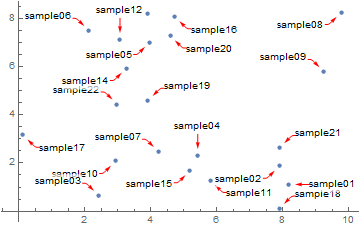
Using Callout:

SeedRandom[1];
data = RandomReal[{0, 10}, {22, 2}];
labels = "sample" <> IntegerString[#, 10, 2] & /@ Range@Length@data;

ListPlot[Callout[#1, #2
    , CalloutStyle -> Red
    , CalloutMarker -> Arrowheads[0.02]
    , LeaderSize -> 15
    ] & @@@ Transpose[{data, labels}]
 , PlotRangePadding -> Scaled[.05]
 ]

enter image description here

$\endgroup$
1
$\begingroup$
SeedRandom[1];

data = RandomReal[{0, 10}, {22, 2}];

keys = "L" <> ToString[#] & /@ Range @ Length @ data;

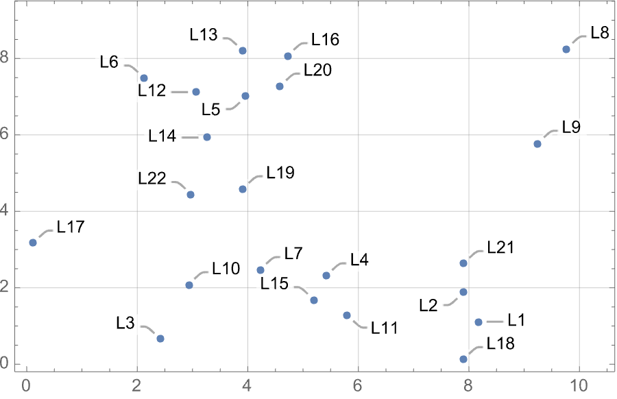
ListPlot automatically places the keys of an Association as labels:

ListPlot[
 AssociationThread[keys -> data],
 Frame -> True,
 GridLines -> Automatic,
 PlotHighlighting -> "Ball"]

enter image description here

$\endgroup$

Your Answer

By clicking “Post Your Answer”, you agree to our terms of service and acknowledge you have read our privacy policy.

Not the answer you're looking for? Browse other questions tagged or ask your own question.