4
$\begingroup$

Here's a simple example of an interpolation function that seems to me to have gone awry. Maybe someone would be so kind as to tell my what's going on with this?

tst2 = {{0, 0}, {0.0057269`, 0.2`}, {0.0366617`, 0.4`}, {0.158682`, 
    0.6`}, {0.50688`, 0.8`}, {0.938627`, 1.`}};

MatrixForm[tst2]
fx = Interpolation[tst2];
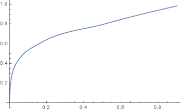
Plot[fx[x], {x, 0.0, 0.9}]

\begin{array}{cc} 0 & 0 \\ 0.0057269 & 0.2 \\ 0.0366617 & 0.4 \\ 0.158682 & 0.6 \\ 0.50688 & 0.8 \\ 0.938627 & 1. \\ \end{array}

Plot of fx[x]

$\endgroup$
6
  • $\begingroup$ All: I know there is a Q&A that already describes the algorithm used by Interpolation that I believe would explain this apparently strange behavior, but I cannot find it. Does anyone recall? $\endgroup$
    – Mr.Wizard
    Commented Jul 14, 2016 at 2:18
  • 2
    $\begingroup$ mathematica.stackexchange.com/questions/4202/… ? $\endgroup$
    – Young
    Commented Jul 14, 2016 at 2:21
  • $\begingroup$ @Young Thanks! I also found this possible duplicate: (104037) $\endgroup$
    – Mr.Wizard
    Commented Jul 14, 2016 at 2:35
  • $\begingroup$ The data doesn't behave much like a polynomial. Perhaps a power law fit will do? Behavior is close to x^.3 $\endgroup$
    – m_goldberg
    Commented Jul 14, 2016 at 3:28
  • $\begingroup$ The suggested vertical asymptote at zero indicates working with the inverse function may be better behaved. $\endgroup$ Commented Jul 14, 2016 at 15:24

5 Answers 5

8
$\begingroup$

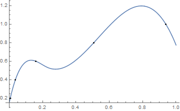
It seems that any InterpolationOrder greater than 1 using the default method (Hermite) yields an unsatisfactory curve.

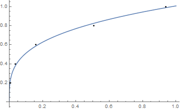
Maybe a simple regression fit would suit your purposes:

tst2 = {{0.0057269, 0.2},{0.0366617, 0.4},{0.158682, 0.6},{0.50688, 0.8}, {0.938627, 1.}};
model = a x^b;
nlm = NonlinearModelFit[tst2, model, {a, b}, x];
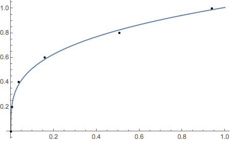
Plot[nlm[x], {x, 0.00, 1}, Epilog -> Point[tst2]]

enter image description here

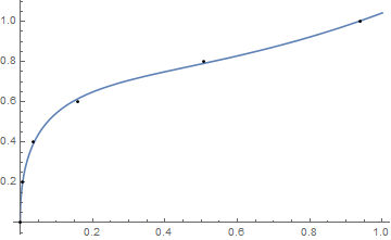
or a more complicated fit:

tst2 = {{0, 0}, {0.0057269, 0.2}, {0.0366617, 0.4}, 
        {0.158682, 0.6}, {0.50688, 0.8}, {0.938627, 1.}};
model = a x^(3/2) - b x + c x^(1/2) + d;
nlm = NonlinearModelFit[tst2, model, {a, b, c, d}, x];
Plot[nlm[x], {x, 0.00, 1}, Epilog -> Point[tst2]]

enter image description here

Example of Method "Spline" at the same order as the default.

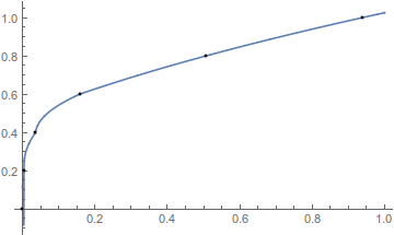
fx = Interpolation[tst2, Method -> "Spline", InterpolationOrder -> 3];
Plot[fx[x], {x, 0.0, 1.0}, Epilog -> Point[tst2]]

enter image description here

Interpolation Reference:

How does Interpolation really work?

$\endgroup$
5
  • $\begingroup$ What version of Mathematica are you using? I am having trouble duplicating your results in V10.4.1 $\endgroup$
    – m_goldberg
    Commented Jul 14, 2016 at 2:50
  • $\begingroup$ Same version, Windows-64bit ... Which graph? $\endgroup$
    – Young
    Commented Jul 14, 2016 at 2:51
  • $\begingroup$ The simple, first one. I'm getting an error message and no evaluation. $\endgroup$
    – m_goldberg
    Commented Jul 14, 2016 at 2:55
  • $\begingroup$ As shown in the answer, I deleted point {0,0} for the simple fit ... {0,0} isn't used in the data set for the last graph either. $\endgroup$
    – Young
    Commented Jul 14, 2016 at 2:57
  • 2
    $\begingroup$ Ah, so. I failed to notice that. Interestingly, NonlinearModelFit[tst2, {a x^b, 0 < b <= .5}, {a, b}, x, Method -> "NMinimize"] works with the original data and gives the same fit as yours. $\endgroup$
    – m_goldberg
    Commented Jul 14, 2016 at 3:02
6
$\begingroup$

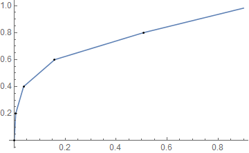
Perhaps linear interpolation will suit your needs:

fx2 = Interpolation[tst2, InterpolationOrder -> 1];

Plot[fx2[x], {x, 0.0, 0.9}, Epilog -> Point[tst2]]

enter image description here

$\endgroup$
6
$\begingroup$

Using the Steffen monotonic interpolation routine from this answer:

tst2 = {{0, 0}, {0.0057269, 0.2}, {0.0366617, 0.4}, {0.158682, 0.6},
        {0.50688, 0.8}, {0.938627, 1.}};
fx = SteffenInterpolation[tst2];

Plot[fx[x], {x, 0.0, 0.9}]

plot of Steffen interpolant

$\endgroup$
2
  • 1
    $\begingroup$ (N.B. Fritsch-Carlson will also work here.) $\endgroup$ Commented Jul 14, 2016 at 2:52
  • $\begingroup$ It's nice to know there even exist such types of interpolation. $\endgroup$
    – Ruslan
    Commented May 23, 2017 at 19:02
3
$\begingroup$

This makes a good fit and includes the point at zero.

data = 
  {{0, 0}, {0.0057269, 0.2}, {0.0366617, 0.4}, {0.158682, 0.6}, {0.50688, 0.8},
   {0.938627, 1.}};
Clear[fx]
fx =
  NonlinearModelFit[data, {a x^b, 0 < b <= .5}, {a, b}, x, 
    Method -> "NMinimize"]["Function"]

1.0077 #1^0.293795 &

Plot[fx[x], {x, 0., 1.},
  Epilog -> {PointSize[Scaled[.01]], Point[data]}]

plot

$\endgroup$
2
  • $\begingroup$ Now that I think about it, OP could probably clarify if what he wants is a fit or an interpolant, as those do different things. $\endgroup$ Commented Jul 14, 2016 at 3:15
  • $\begingroup$ @J.M. Good point, but there a 3rd position on the matter: doesn't care which. Perhaps you make a query to the OP on this as a comment to the question. $\endgroup$
    – m_goldberg
    Commented Jul 14, 2016 at 3:23
0
$\begingroup$

Following up on my comment about inverse functions, a simple implementation ...

tst2 = {{0, 0}, {0.0057269`, 0.2`}, {0.0366617`, 0.4`}, {0.158682`, 0.6`}, {0.50688`, 0.8`}, {0.938627`, 1.`}};
ifx = Interpolation[Reverse /@ tst2];
fx = InverseFunction[FunctionInterpolation[ifx[y], {y, 0, 1}]];
Plot[fx[x], {x, 0, 1}, Epilog -> Point[tst2]]

Mathematica graphics

$\endgroup$

Your Answer

By clicking “Post Your Answer”, you agree to our terms of service and acknowledge you have read our privacy policy.

Not the answer you're looking for? Browse other questions tagged or ask your own question.