replaced http://mathematica.stackexchange.com/ with https://mathematica.stackexchange.com/
Source Link

It seems that any InterpolationOrder greater than 1 using the default method (Hermite) yields an unsatisfactory curve.

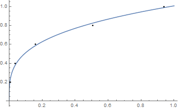
Maybe a simple regression fit would suit your purposes:

tst2 = {{0.0057269, 0.2},{0.0366617, 0.4},{0.158682, 0.6},{0.50688, 0.8}, {0.938627, 1.}};
model = a x^b;
nlm = NonlinearModelFit[tst2, model, {a, b}, x];
Plot[nlm[x], {x, 0.00, 1}, Epilog -> Point[tst2]]

enter image description here

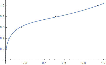
or a more complicated fit:

tst2 = {{0, 0}, {0.0057269, 0.2}, {0.0366617, 0.4}, 
        {0.158682, 0.6}, {0.50688, 0.8}, {0.938627, 1.}};
model = a x^(3/2) - b x + c x^(1/2) + d;
nlm = NonlinearModelFit[tst2, model, {a, b, c, d}, x];
Plot[nlm[x], {x, 0.00, 1}, Epilog -> Point[tst2]]

enter image description here

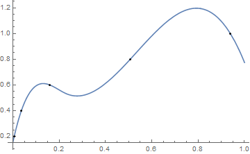
Example of Method "Spline" at the same order as the default.

fx = Interpolation[tst2, Method -> "Spline", InterpolationOrder -> 3];
Plot[fx[x], {x, 0.0, 1.0}, Epilog -> Point[tst2]]

enter image description here

Interpolation Reference:

How does Interpolation really work?How does Interpolation really work?

It seems that any InterpolationOrder greater than 1 using the default method (Hermite) yields an unsatisfactory curve.

Maybe a simple regression fit would suit your purposes:

tst2 = {{0.0057269, 0.2},{0.0366617, 0.4},{0.158682, 0.6},{0.50688, 0.8}, {0.938627, 1.}};
model = a x^b;
nlm = NonlinearModelFit[tst2, model, {a, b}, x];
Plot[nlm[x], {x, 0.00, 1}, Epilog -> Point[tst2]]

enter image description here

or a more complicated fit:

tst2 = {{0, 0}, {0.0057269, 0.2}, {0.0366617, 0.4}, 
        {0.158682, 0.6}, {0.50688, 0.8}, {0.938627, 1.}};
model = a x^(3/2) - b x + c x^(1/2) + d;
nlm = NonlinearModelFit[tst2, model, {a, b, c, d}, x];
Plot[nlm[x], {x, 0.00, 1}, Epilog -> Point[tst2]]

enter image description here

Example of Method "Spline" at the same order as the default.

fx = Interpolation[tst2, Method -> "Spline", InterpolationOrder -> 3];
Plot[fx[x], {x, 0.0, 1.0}, Epilog -> Point[tst2]]

enter image description here

Interpolation Reference:

How does Interpolation really work?

added 405 characters in body
Source Link
Young
  • 7.5k
  • 1
  • 22
  • 46

It seems that any InterpolationOrder greater than 1 using the default method (Hermite) yields an unsatisfactory curve.

Maybe a simple regression fit would suit your purposes:

tst2 = {{0.0057269, 0.2},{0.0366617, 0.4},{0.158682, 0.6},{0.50688, 0.8}, {0.938627, 1.}};
model = a x^b;
nlm = NonlinearModelFit[tst2, model, {a, b}, x];
Plot[nlm[x], {x, 0.00, 1}, Epilog -> Point[tst2]]

enter image description here

or a more complicated fit:

tst2 = {{0, 0}, {0.0057269, 0.2}, {0.0366617, 0.4}, 
        {0.158682, 0.6}, {0.50688, 0.8}, {0.938627, 1.}};
model = a x^(3/2) - b x + c x^(1/2) + d;
nlm = NonlinearModelFit[tst2, model, {a, b, c, d}, x];
Plot[nlm[x], {x, 0.00, 1}, Epilog -> Point[tst2]]

enter image description here

Example of Method "Spline" at the same order as the default.

fx = Interpolation[tst2, Method -> "Spline", InterpolationOrder -> 3];
Plot[fx[x], {x, 0.0, 1.0}, Epilog -> Point[tst2]]

enter image description here

Interpolation Reference:

How does Interpolation really work?

It seems that any InterpolationOrder greater than 1 using the default method (Hermite) yields an unsatisfactory curve.

Maybe a simple regression fit would suit your purposes:

tst2 = {{0.0057269, 0.2},{0.0366617, 0.4},{0.158682, 0.6},{0.50688, 0.8}, {0.938627, 1.}};
model = a x^b;
nlm = NonlinearModelFit[tst2, model, {a, b}, x];
Plot[nlm[x], {x, 0.00, 1}, Epilog -> Point[tst2]]

enter image description here

or more complicated fit:

tst2 = {{0, 0}, {0.0057269, 0.2}, {0.0366617, 0.4}, 
        {0.158682, 0.6}, {0.50688, 0.8}, {0.938627, 1.}};
model = a x^(3/2) - b x + c x^(1/2) + d;
nlm = NonlinearModelFit[tst2, model, {a, b, c, d}, x];
Plot[nlm[x], {x, 0.00, 1}, Epilog -> Point[tst2]]

enter image description here

Example of Method "Spline" at the same order as the default.

fx = Interpolation[tst2, Method -> "Spline", InterpolationOrder -> 3];
Plot[fx[x], {x, 0.0, 1.0}, Epilog -> Point[tst2]]

enter image description here

Interpolation Reference:

How does Interpolation really work?

It seems that any InterpolationOrder greater than 1 using the default method (Hermite) yields an unsatisfactory curve.

Maybe a simple regression fit would suit your purposes:

tst2 = {{0.0057269, 0.2},{0.0366617, 0.4},{0.158682, 0.6},{0.50688, 0.8}, {0.938627, 1.}};
model = a x^b;
nlm = NonlinearModelFit[tst2, model, {a, b}, x];
Plot[nlm[x], {x, 0.00, 1}, Epilog -> Point[tst2]]

enter image description here

or a more complicated fit:

tst2 = {{0, 0}, {0.0057269, 0.2}, {0.0366617, 0.4}, 
        {0.158682, 0.6}, {0.50688, 0.8}, {0.938627, 1.}};
model = a x^(3/2) - b x + c x^(1/2) + d;
nlm = NonlinearModelFit[tst2, model, {a, b, c, d}, x];
Plot[nlm[x], {x, 0.00, 1}, Epilog -> Point[tst2]]

enter image description here

Example of Method "Spline" at the same order as the default.

fx = Interpolation[tst2, Method -> "Spline", InterpolationOrder -> 3];
Plot[fx[x], {x, 0.0, 1.0}, Epilog -> Point[tst2]]

enter image description here

Interpolation Reference:

How does Interpolation really work?

added 405 characters in body
Source Link
Young
  • 7.5k
  • 1
  • 22
  • 46

It seems that any InterpolationOrder greater than 1 using the default method (Hermite) yields an unsatisfactory curve.

Maybe a simple regression fit would suit your purposes:

tst2 = {{0.0057269, 0.2},{0.0366617, 0.4},{0.158682, 0.6},{0.50688, 0.8}, {0.938627, 1.}};
model = a x^b;
nlm = NonlinearModelFit[tst2, model, {a, b}, x];
Plot[nlm[x], {x, 0.00, 1}, Epilog -> Point[tst2]]

enter image description here

or more complicated fit:

tst2 = {{0, 0}, {0.0057269, 0.2}, {0.0366617, 0.4}, 
        {0.158682, 0.6}, {0.50688, 0.8}, {0.938627, 1.}};
model = a x^(3/2) - b x + c x^(1/2) + d;
nlm = NonlinearModelFit[tst2, model, {a, b, c, d}, x];
Plot[nlm[x], {x, 0.00, 1}, Epilog -> Point[tst2]]

enter image description here

Example of Method "Spline" at the same order as the default.

fx = Interpolation[tst2, Method -> "Spline", InterpolationOrder -> 3];
Plot[fx[x], {x, 0.0, 1.0}, Epilog -> Point[tst2]]

enter image description here

Interpolation Reference:

How does Interpolation really work?

It seems that any InterpolationOrder greater than 1 using the default method (Hermite) yields an unsatisfactory curve.

Maybe a regression fit would suit your purposes:

tst2 = {{0.0057269, 0.2},{0.0366617, 0.4},{0.158682, 0.6},{0.50688, 0.8}, {0.938627, 1.}};
model = a x^b;
nlm = NonlinearModelFit[tst2, model, {a, b}, x];
Plot[nlm[x], {x, 0.00, 1}, Epilog -> Point[tst2]]

enter image description here

Example of Method "Spline" at the same order as the default.

fx = Interpolation[tst2, Method -> "Spline", InterpolationOrder -> 3];
Plot[fx[x], {x, 0.0, 1.0}, Epilog -> Point[tst2]]

enter image description here

Interpolation Reference:

How does Interpolation really work?

It seems that any InterpolationOrder greater than 1 using the default method (Hermite) yields an unsatisfactory curve.

Maybe a simple regression fit would suit your purposes:

tst2 = {{0.0057269, 0.2},{0.0366617, 0.4},{0.158682, 0.6},{0.50688, 0.8}, {0.938627, 1.}};
model = a x^b;
nlm = NonlinearModelFit[tst2, model, {a, b}, x];
Plot[nlm[x], {x, 0.00, 1}, Epilog -> Point[tst2]]

enter image description here

or more complicated fit:

tst2 = {{0, 0}, {0.0057269, 0.2}, {0.0366617, 0.4}, 
        {0.158682, 0.6}, {0.50688, 0.8}, {0.938627, 1.}};
model = a x^(3/2) - b x + c x^(1/2) + d;
nlm = NonlinearModelFit[tst2, model, {a, b, c, d}, x];
Plot[nlm[x], {x, 0.00, 1}, Epilog -> Point[tst2]]

enter image description here

Example of Method "Spline" at the same order as the default.

fx = Interpolation[tst2, Method -> "Spline", InterpolationOrder -> 3];
Plot[fx[x], {x, 0.0, 1.0}, Epilog -> Point[tst2]]

enter image description here

Interpolation Reference:

How does Interpolation really work?

added 256 characters in body
Source Link
Young
  • 7.5k
  • 1
  • 22
  • 46
Loading
Source Link
Young
  • 7.5k
  • 1
  • 22
  • 46
Loading