Findfit does not find the best fit

Question

I am working on a project that needs curve fitting. The experimental data should be fitted with a model that calculated with an integration equation. At first, I enter my experimental data

    ClearAll[data, L, P, z0, alpha0, Leff, landa, w0, w, I0, II, q, Q, T, t, z, beta, Is];
data = {{-11.`, 0.989518737`}, {-10.8`, 0.986423266`}, {-10.6`, 
0.988486913`}, {-10.4`, 0.988486913`}, {-10.2`, 
0.98745509`}, {-10.`, 0.988486913`}, {-9.8`, 
0.988486913`}, {-9.6`, 0.99055056`}, {-9.4`, 0.98745509`}, {-9.2`,
 0.984359619`}, {-9.`, 0.989518737`}, {-8.8`, 
0.983327796`}, {-8.6`, 0.98745509`}, {-8.4`, 
0.984359619`}, {-8.2`, 0.992614207`}, {-8.`, 
0.996741501`}, {-7.8`, 0.996741501`}, {-7.6`, 
0.989518737`}, {-7.4`, 0.991582384`}, {-7.2`, 
0.998805148`}, {-7.`, 0.996741501`}, {-6.8`, 
0.995709678`}, {-6.6`, 0.995709678`}, {-6.4`, 
0.994677854`}, {-6.2`, 1.001900619`}, {-6.`, 1.00809156`}, {-5.8`,
 1.006027913`}, {-5.6`, 1.009123383`}, {-5.4`, 
0.996741501`}, {-5.2`, 0.994677854`}, {-5.`, 
1.018409795`}, {-4.8`, 1.020473442`}, {-4.6`, 
1.023568912`}, {-4.4`, 1.024600736`}, {-4.2`, 
1.027696206`}, {-4.`, 1.030791677`}, {-3.8`, 
1.033887147`}, {-3.6`, 1.030791677`}, {-3.4`, 
1.02872803`}, {-3.2`, 1.0318235`}, {-3.`, 1.036982618`}, {-2.8`, 
1.041109912`}, {-2.6`, 1.042141735`}, {-2.4`, 
1.038014441`}, {-2.2`, 1.034918971`}, {-2.`, 1.0318235`}, {-1.8`, 
1.024600736`}, {-1.6`, 1.014282501`}, {-1.4`, 
1.004996089`}, {-1.2`, 0.994677854`}, {-1.`, 
0.980232325`}, {-0.8`, 0.960627679`}, {-0.6`, 
0.936895738`}, {-0.4`, 0.909036504`}, {-0.2`, 0.886336387`}, {0.`,
 0.865699917`}, {0.2`, 0.860540799`}, {0.4`, 0.883240916`}, {0.6`,
 0.936895738`}, {0.8`, 0.981264149`}, {1.`, 0.991582384`}, {1.2`, 
1.026664383`}, {1.4`, 1.033887147`}, {1.6`, 1.046269029`}, {1.8`, 
1.036982618`}, {2.`, 1.044205382`}, {2.2`, 1.041109912`}, {2.4`, 
1.0318235`}, {2.6`, 1.030791677`}, {2.8`, 1.026664383`}, {3.`, 
1.030791677`}, {3.2`, 1.032855324`}, {3.4`, 1.0318235`}, {3.6`, 
1.027696206`}, {3.8`, 1.02872803`}, {4.`, 1.023568912`}, {4.2`, 
1.020473442`}, {4.4`, 1.015314324`}, {4.6`, 1.013250677`}, {4.8`, 
1.013250677`}, {5.`, 1.009123383`}, {5.2`, 1.007059736`}, {5.4`, 
1.006027913`}, {5.6`, 1.004996089`}, {5.8`, 1.006027913`}, {6.`, 
1.003964266`}, {6.2`, 1.002932442`}, {6.4`, 1.000868795`}, {6.6`, 
0.998805148`}, {6.8`, 0.999836972`}, {7.`, 0.996741501`}, {7.2`, 
0.993646031`}, {7.4`, 0.992614207`}, {7.6`, 0.99055056`}, {7.8`, 
0.991582384`}, {8.`, 0.989518737`}, {8.2`, 0.988486913`}, {8.4`, 
0.98745509`}, {8.6`, 0.985391443`}, {8.8`, 0.986423266`}, {9.`, 
0.985391443`}};

The initial value of some variables are:

L = 0.12;
P = 0.035;
z0 = 0.8;
alpha0 = 3.4302;

And some other functions and variables are built as:

Leff = (1 - E^(-alpha0*L))/alpha0;
landa = 532*10^-7;
w0 = Sqrt[(landa*z0)/Pi];
w[z_] = w0*Sqrt[1 + (z/z0)^2];
I0 = (2*P)/(Pi*w0^2);
II[z_] = (2*P)/(Pi*(w[z])^2);
q[z_, beta_] = (beta*I0*Leff)/(1 + (z/z0)^2);
Q[z_, Is_] = Exp[(alpha0*L*II[z])/(II[z] + Is)];

And at last the model equation is built as:

T[(beta_)?NumericQ, (Is_)?NumericQ, (z_)?NumericQ] = Q[z, Is]/(Sqrt[Pi]*q[z, beta])*NIntegrate[Log[1 + q[z, beta]*Exp[-t^2]], {t, -\[Infinity], \[Infinity]}];

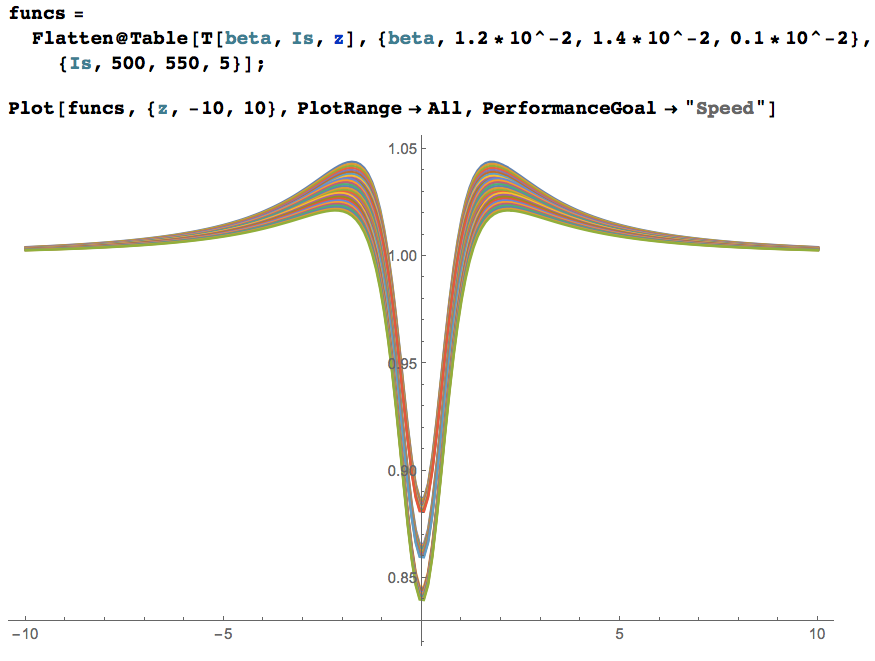
Now we have FindFit to find beta and Is: (the range of beta and Is are obtained by repeat the code to find a curve fitting near the experimental data, and if any other range results better fitting so that will be accepted.)

fit = FindFit[data, {T[beta, Is, z], 1.2*10^-2 < beta < 1.4*10^-2,500 < Is <550}, {beta, Is}, z]
Show[Plot[T[beta, Is, z] /. fit, {z, -11, 9}, PlotRange -> All],ListPlot[data]]

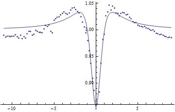
And the result is:

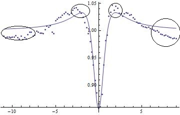
I expect that the regions shown below, should have the better agreement:

I really thank you if you could help or guide me to have a better result.

Answer 1

It seems it is better to use a family of functions instead of just one. The code below uses NonLinearFit instead of FindFit, since I do not think using FindFit is a hard requirement in the question.

Also, below I assume that the definitions in the question are evaluated.

First, let us speed-up the use of NIntegrate:

T[(beta_)?NumericQ, (Is_)?NumericQ, (z_)?NumericQ] := 
  Q[z, Is]/(Sqrt[Pi]*q[z, beta])*
   NIntegrate[
    Log[1 + q[z, beta]*Exp[-t^2]], {t, -\[Infinity], \[Infinity]}, 
    PrecisionGoal -> 3, 
    Method -> {Automatic, "SymbolicProcessing" -> 0}];

Second, let us select and plot a family of functions:

funcs = Flatten@
   Table[T[beta, Is, z], {beta, 1.2*10^-2, 1.4*10^-2, 0.1*10^-2}, {Is, 500, 550, 5}];

Plot[funcs, {z, -10, 10}, PlotRange -> All, 
 PerformanceGoal -> "Speed"]

(I selected the functions using the ranges of the parameters given to FindFit in the question.)

Next we create linear combinations variables:

vars = Array[a, Length[funcs]];

...and do a model fit:

fm = NonlinearModelFit[data, vars.funcs, vars, z, 
  Method -> "NMinimize"]

Notice the choice of the method. With the default method I was getting singular curves (which were still providing a good fit).

Finally, we plot the data and the model function:

Show[ListPlot[data], 
 Plot[fm[x], {x, -10, 10}, PerformanceGoal -> "Speed"]]

This question and my response are very similar to Non-linear curve fit problem.