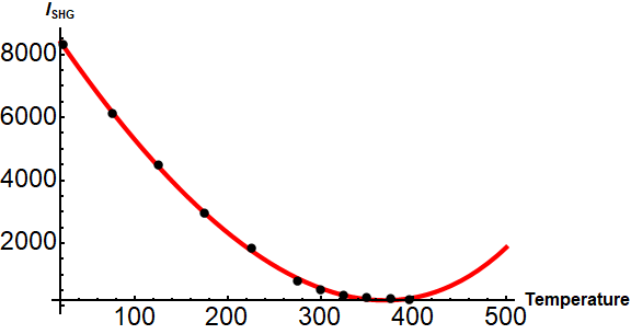
I'm having trouble fitting this transition temperature equation to my data. Physically speaking, the intensity should flatten out for T>Tc, which seems to be the biggest problem here. The equation I've chosen to fit (SHGfit) uses a generic polarization as a function of temperature P[T_,B_,Tc], and an additional contribution to the measured intensity, an arbitrary B*Exp[I*\[Phi]] phase shift. I keep getting the error that the NonlinearModelFit did not converge, but the fit looks very close to working, or at least converging.
Modsq[z_] := ComplexExpand[Re[z]]^2 + ComplexExpand[Im[z]]^2;
SHGfit[A_, P_, B_, \[Phi]_] := Modsq[A*P + B*Exp[I*\[Phi]]]
P[T_, B_, Tc_] := 1/(T - Tc)^B

data={{22, 8325.33}, {75, 6112.66}, {125, 4495.},
  {175, 2948.66}, {225, 1847.66}, {275, 798.33},
   {300, 504.}, {325, 357.}, {350, 279.66}, {375, 223.}, {395, 192.}}

g = NonlinearModelFit[data, {SHGfit[A, P[t, \[Gamma], Tc], B, \[Phi]], \[Gamma] < 0, Tc > 300},
    {{A, -0.7}, {\[Gamma], -0.8}, {\[Phi], 2.29}, {Tc, 379}, {B, -34.8}}, t,
    WorkingPrecision -> 25];
Show[Plot[g[t], {t, 20, 500}, PlotRange -> All, PlotStyle -> {Red, Thickness[0.01]},
   AxesStyle -> {{Thick, Black}, {Thick, Black}},
   TicksStyle -> {{Large, Black}, {Large, Black}},
   AxesLabel -> {Style["Temperature", Bold, 16],
     Style["\!\(\*SubscriptBox[\(I\), \(SHG\)]\)", Bold, 16]}, ImageSize -> Large],
  ListPlot[data, PlotStyle -> {PointSize[0.02], Black}]]
Is there anything obvious that I'm doing wrong? I would really appreciate some advice on nonlinear fitting. Thanks!
EDIT: I realized that my data points were a bit sparse so here is a fuller data set:
{{30, 8782}, {40, 8674}, {50, 8313}, {60, 8016}, {70, 7577}, {80, 7368}, {90, 6930}, {100, 6447}, {110, 6111}, {120, 5673}, {130, 5321}, {140, 5019}, {150, 4680}, {160, 4311}, {170, 3985}, {180, 3593}, {190, 3290}, {200, 2983}, {210, 2640}, {220, 2408}, {230, 2059}, {240, 1837}, {250, 1526}, {260, 1198}, {270, 918}, {280, 638}, {290, 402}, {300, 258}, {310, 184}, {320, 140}, {330, 113}, {340, 98}, {350, 86}, {360, 75}, {370, 66}, {380, 62}, {390, 54}, {400, 51}}
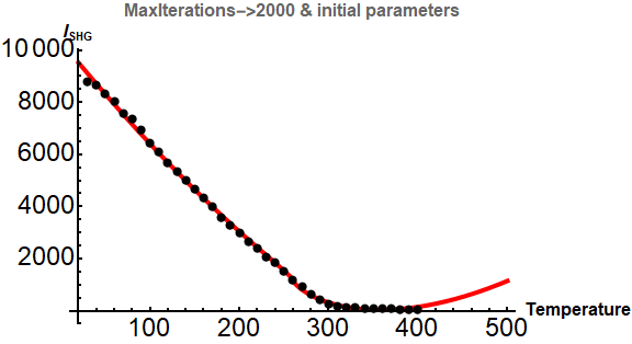
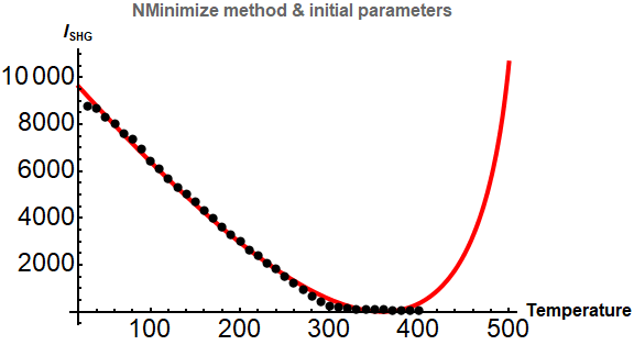
And implementing a couple new ideas (thank you JimB and Ulrich Neumann) such as setting MaxIterations->2000 and Model->"NMinimize" yield the following converging fits, although they physically don't describe the temperature dependence, which should flatten out to a constant at higher temperatures. 

From here, I guess it's a matter of choosing the correct physical constraints?


N[g["CorrelationMatrix"] // MatrixForm, 5]contains correlation coefficients are are all nearly 1.0 in magnitude. Another indication of this is that the standard errors of all parameters are huge compared to the estimates resulting in nearly all of the P-values being very close to 1. $\endgroup$data=Rationalize[data,0]and adding inMaxIterations->2000toNonlinearModelFit. Then the correlation matrix looks much better and the standard errors for the parameters are much, much smaller. $\endgroup$