3
$\begingroup$

I am having a problem with making a fit to data in Mathematica, which may involve my understanding of the methods available.

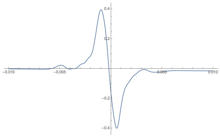
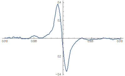
I am trying to fit the derivative of a Frota function (which is a Single Peak curve) together with two Gaussian Amplitudes.

The raw data looks loke this: enter image description here

In theory, the Frota function can be described as:

f[V_, phi_, gamma_, ek_, a_, b_, c_] := 
   a*Im[E^(I*phi)*Sqrt[(I*gamma)/(V - ek + I*gamma)]] + b*V + c;

As you can see that is not a function that can be differentiated easily. First I tried to differentiated it in the following way:

df[V_, phi_, gamma_, ek_, a_, b_, c_] := 
  D[ComplexExpand[f[x, phi, gamma, ek, a, b, c]], x] /. x -> V;
df[V, phi, gamma, ek, a, b, c]

In principle that works, but the function f has to be complex expanded before taking the derivative, due to the imaginary part not having a non numeric derivative. Moreover, when I plot the function, I have to take the real part. Still I get reasonable results and can fit my data with the function:

dfP2Gauss[V_, phi_, gamma_, ek_, a_, b_, c_, Agauss1_, Agauss2_, 
          Gcenter1_, Gcenter2_, gGauss1_, gGauss2_] := 
  df[V, phi, gamma, ek, a, b, c] + 
  (c + Agauss1*E^(-0.5 ((V - center1)/ gGauss1)^2)) + 
  (c + Agauss2*E^(-0.5 ((V + Gcenter2)/ gGauss2)^2))

where I put some the Gaussian peaks in.

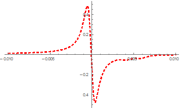
enter image description here

That does not look to bad, but when I start to fit my data (which consists of around 200 points), it takes like 40 minutes to do 100 iteration. Further, it gives bad results, because it makes the Gaussian peaks almost zero, even when I give good starting parameters. I also tried to make borders for the widths of the Gaussians, but then it just stays at the lower limit. Because of the incredible long caluculation time, I can't increase the iterations to say 1000, and even if did I don't it would help much. Maybe someone can help me?

Furthermore, I tried to calculate the derivative numerically:

numericfrota[V_, phi_, gamma_, ek_, a_, b_, c_, y0_] := 
  ND[f[V, phi, gamma, ek, a, b, c], V, y0, Terms -> 30]

The calculation of the derivative now goes four times faster, but I can't plot it together with the Gaussians.

My code would be something like this:

numericGauss[V_, phi_, gamma_, ek_, a_, b_, c_, y0_, Agauss1_, 
             Agauss2_, Gcenter1_, Gcenter2_, gGauss1_, gGauss2_] := 
  numericfrota[V, phi, gamma, ek, a, b, c, y0] + 
  (c + Agauss1*E^(-0.5 ((V - Gcenter1)/ gGauss1)^2)) + 
  (c + Agauss2*E^(-0.5 ((V + Gcenter2)/ gGauss2)^2));

But when I try to evaluate this, I need to give to specifications, y0 and V. They need to be the same and go from -0.01 and 0.01. But Mathematica just allows me to give one range, either y0 and V. If I choose to just take V and, therefore, derive the numeric Frota in respect of V at the point V, I just get a straight line. I just don't know how to properly adjust my functions.

$\endgroup$
4
  • 3
    $\begingroup$ Is it possible to provide the 200 data points referred to in the question? $\endgroup$ Commented Sep 28, 2015 at 15:33
  • $\begingroup$ Do you need to fit the Frota funciton derivative or any approximation/interpolation would work? $\endgroup$ Commented Sep 28, 2015 at 18:12
  • $\begingroup$ I agree that the data would be essential. But also with the original Frota function having but a single having a single peak, why not fit that curve and then take the derivative of the fitted curve? I ask because is the dependent variable a measured rate of change (i.e., the derivative) or the value of the Frota function? $\endgroup$
    – JimB
    Commented Sep 28, 2015 at 20:23
  • $\begingroup$ You showed a plot of df with some noise but didn't supply the phi, gamma, ek, etc, parameters you used. Could you supply those parameters? $\endgroup$ Commented Sep 29, 2015 at 22:45

1 Answer 1

8
$\begingroup$

I am not sure how useful my answer is, but I hope it will bring some points to be clarified in the question. (Also I spent some time on this so I wanna proclaim some of the results of my efforts...)

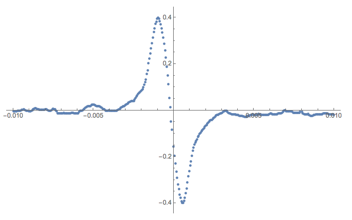
Since the data was not provided in the original question I extracted it from the image shown following the (great) explanations here: Recovering data points from an image.

Here is a plot with the extracted points:

enter image description here

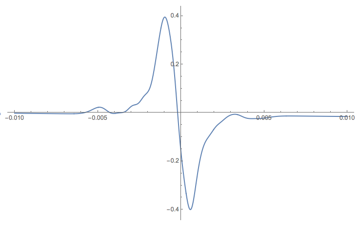
Next, I just used Chebyshev polynomials to find a fit with the following commands:

fit = Fit[data, ChebyshevT[#, 90. x] & /@ Range[0, 40], x];
Plot[fit, {x, Min[data[[All, 1]]], Max[data[[All, 1]]]}, PlotRange -> All]

enter image description here

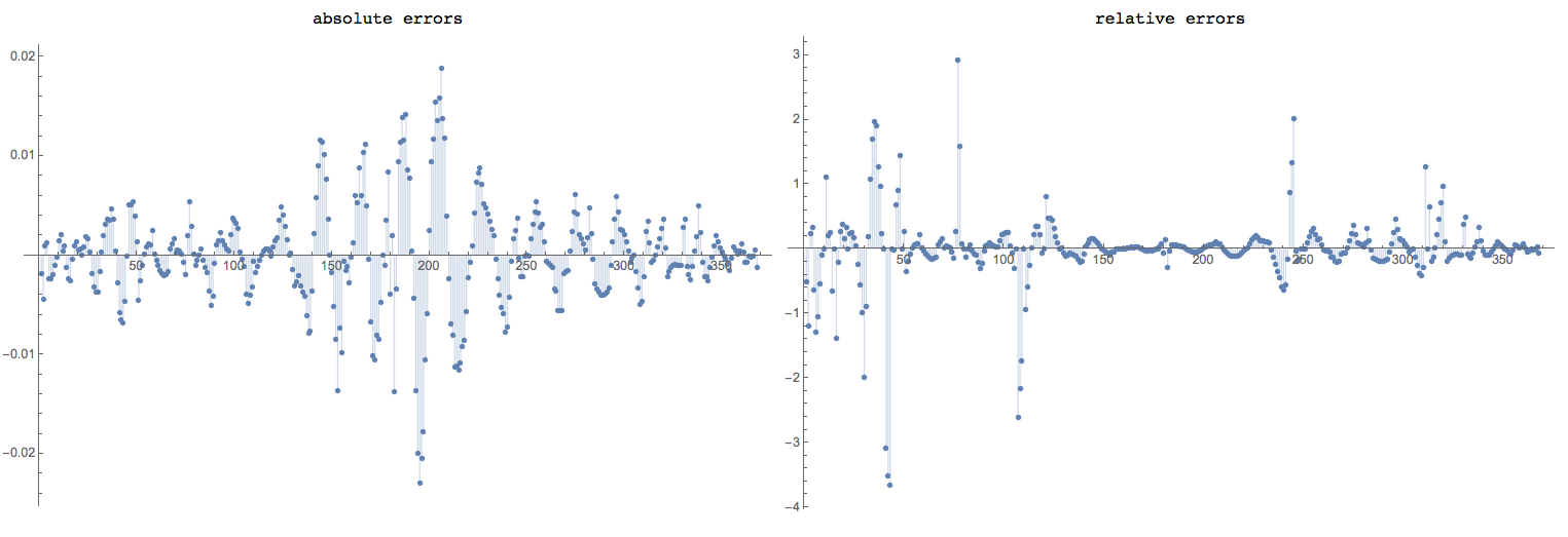
Here are the errors:

opts = {Filling -> Axis, PlotRange -> All, ImageSize -> 600};
Grid[{{"absolute errors", "relative errors"},
  {ListPlot[Map[(#[[2]] - (fit /. x -> #[[1]])) &, data], opts],
   ListPlot[
    Map[(#[[2]] - (fit /. x -> #[[1]]))/(Abs[#[[2]]] /. {0. -> 1}) &, 
     data], opts]}}]

enter image description here

If I understand the question correctly the fitting of a particular type of family of curves is desired. I was not able to work with the functions provided in the question. I used SkewNormalDistribution PDF that seems to have similar properties as the data. So I repeated the above commands using a generated basis of SkewNormalDistribution PDF's derived with combinations of different parameters ranges. I assume this approach would work with the functions in the question.

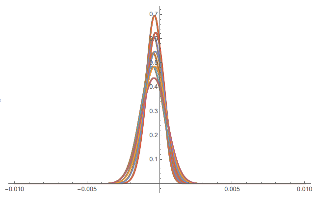
First we generate around 100 functions and plot them:

funcs = Flatten@
   Table[PDF[SkewNormalDistribution[c, s, \[Alpha]], 
      x] /. {x -> ( x*1000)}, {\[Alpha], {-1, -0.6}}, {c, -0.04, 0.01,0.004}, {s, 0.7, 1, 0.1}];
Plot[Evaluate@funcs, {x, Min[data[[All, 1]]], Max[data[[All, 1]]]}, 
 PlotRange -> All]

enter image description here

Note that I have chosen the peaks locations and the scale factor for x according to the peaks and spread in the experimental data.

Next using the generated functions we add to them their antisymmetric versions and {1,x,-x}. The resulted list is given to Fit:

fn = Fit[data, Join[{1, x, -x}, funcs, -funcs /. {x -> (-x)}], x];

Plot[fn, {x, Min[data[[All, 1]]], Max[data[[All, 1]]]}, 
 PlotRange -> All]

enter image description here

Here are the errors:

opts = {Filling -> Axis, PlotRange -> All, ImageSize -> 600};
Grid[{{"absolute errors", "relative errors"},
  {ListPlot[Map[(#[[2]] - (fn /. x -> #[[1]])) &, data], opts],
   ListPlot[
    Map[(#[[2]] - (fn /. x -> #[[1]]))/(Abs[#[[2]]] /. {0. -> 1}) &, 
     data], opts]}}]

enter image description here

$\endgroup$

Your Answer

By clicking “Post Your Answer”, you agree to our terms of service and acknowledge you have read our privacy policy.

Not the answer you're looking for? Browse other questions tagged or ask your own question.