5
$\begingroup$

Thank you everyone for your meaningful contributions!

My Goal and Problem
I'm trying to fit a particular ODE in a set of ODE's to experimental data. I've attempted to implement this by following the examples listed below to no avail:

My Approach
I was originally having problems fitting the data because of bad initial guesses, so I've implemented a plot to manipulate the original parameters. This would give me a good initial guess to input into the minimization function. Here is the code:

data = {{94.30210177`, 0.864346486`}, {95.32514753`, 
    0.859754108`}, {96.34819329`, 0.854044984`}, {97.37123904`, 
    0.847107439`}, {98.30903099`, 0.839836015`}, {99.16156912`, 
    0.83232005`}, {99.92885344`, 0.823816908`}, {100.6108839`, 
    0.816520995`}, {101.2929145`, 0.808806302`}, {101.974945`, 
    0.800254051`}, {102.5717216`, 0.793411563`}, {103.1684983`, 
    0.784240661`}, {103.765275`, 0.77655503`}, {104.3620517`, 
    0.768897318`}, {104.9588284`, 0.760681234`}, {105.5556051`, 
    0.752716417`}, {106.2376356`, 0.744917968`}, {106.9196661`, 
    0.736365717`}, {107.6016966`, 0.727980977`}, {108.2837271`, 
    0.719428725`}, {108.9657576`, 0.711211497`}, {109.733042`, 
    0.702269474`}, {110.3298186`, 0.694721203`}, {111.0409556`, 
    0.687875903`}, {111.41376`, 0.680476135`}, {112.2054025`, 
    0.672472809`}, {112.9726869`, 0.664086925`}, {113.6547174`, 
    0.655255487`}, {114.1662402`, 0.648548153`}, {114.7630169`, 
    0.639606183`}, {115.3597936`, 0.63032919`}, {115.9736211`, 
    0.622771757`}, {116.485144`, 0.614992346`}, {116.9284638`, 
    0.60721385`}, {117.491139`, 0.598194166`}, {117.9856111`, 
    0.589510421`}, {118.5312355`, 0.580256448`}, {119.0257076`, 
    0.570534129`}, {119.7077381`, 0.561144318`}, {120.3897686`, 
    0.553429626`}, {121.1570529`, 0.545914804`}, {122.0948449`, 
    0.53833069`}, {123.1178906`, 0.532286543`}, {124.1409364`, 
    0.526689093`}, {125.1639821`, 0.520979969`}, {126.1870279`, 
    0.515829218`}, {127.2100737`, 0.510343443`}, {128.2331194`, 
    0.504745993`}, {129.2561652`, 0.500153615`}, {130.2792109`, 
    0.496231284`}, {131.3022567`, 0.492197279`}, {132.3253024`, 
    0.487939924`}, {133.3483482`, 0.484240942`}, {134.371394`, 
    0.480095262`}, {135.3944397`, 0.476284606`}, {136.4174855`, 
    0.473032322`}, {137.389379`, 0.469445701`}, {138.463577`, 
    0.463735891`}, {139.4866228`, 0.458808489`}, {140.5096685`, 
    0.454327785`}, {141.5327143`, 0.449735406`}, {142.55576`, 
    0.445366377`}, {143.5788058`, 0.440997348`}, {144.6018515`, 
    0.436069946`}, {145.6248973`, 0.431477568`}, {146.6479431`, 
    0.42666184`}, {147.6709888`, 0.421957787`}, {148.6940346`, 
    0.417700432`}, {149.5749906`, 0.414785078`}, {150.9106337`, 
    0.411863626`}, {151.9336795`, 0.409951437`}, {152.9567252`, 
    0.407257526`}, {153.979771`, 0.40467529`}, {155.0028168`, 
    0.402539752`}};

Rg = 8.314*10^-3;
HR = 5;
n1 = 1;
n2 = 1.5;
n3 = 1.5;
T = HR*t + T0;

system = {Cb'[t] == -a1*E^(-e1/(Rg*T))*(Cb[t]^n1), 
   Cbp'[t] == 
    a1*E^(-e1/(Rg*T))*(Cb[t]^n1) - a2*E^(-e2/(Rg*T))*(Cbp[t]^n2) - 
     a3*E^(-e3/(Rg*T))*(Cbp[t]^n3), 
   Cg'[t] == a2*E^(-e2/(Rg*T))*Cbp[t]^n2, 
   Cc'[t] == a3*E^(-e3/(Rg*T))*Cbp[t]^n3, Cb[0] == 1, Cbp[0] == 0, 
   Cg[0] == 0, Cc[0] == 0};

sol = ParametricNDSolveValue[
   system, {Cb, Cbp, Cg, Cc}, {t, 0, 180}, {a1, e1, a2, e2, a3, e3, 
    T0}];

Manipulate[
 Show[
  Plot[Evaluate@Through[sol[a1, e1, a2, e2, a3, e3, T0][t]], {t, 0, 
    180}, PlotLegends -> {"Cb[t]", "Cb+[t]", "Cg[t]", "Cc[t]"}, 
   AxesLabel -> Automatic],
  ListPlot[data, PlotStyle -> {PointSize[Small], Black}]
  ],
 {{a1, 1.855}, .5, 5, Appearance -> "Labeled"}, {{e1, 2.35}, 0, 10, 
  Appearance -> "Labeled"}, {{a2, 4.15}, 0, 7, 
  Appearance -> "Labeled"}, {{e2, 41.9}, 15, 80, 
  Appearance -> "Labeled"}, {{a3, 5.13}, 0, 8, 
  Appearance -> "Labeled"}, {{e3, 45.3}, 15, 80, 
  Appearance -> "Labeled"}, {{T0, 290}, 273, 320, 
  Appearance -> "Labeled"}]

This gives a nice plot I can manipulate as shown below (Black points are experimental data): nice plot, man
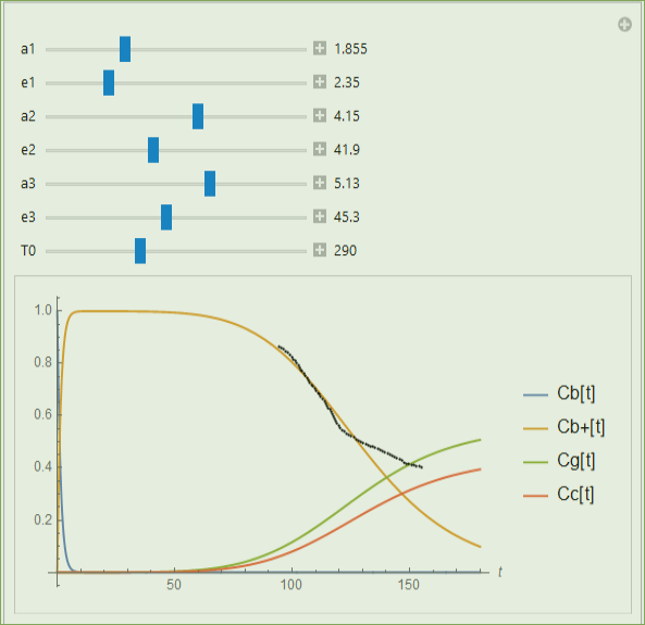
My Approach at the Solution
So, I have now tried to use the parameters to drive the minimization of matching the Cb+ curve to the data. I would like the best fit for that curve, and how it effects the parameters of the other curves I am less concerned with.

First I created a model that takes uses

model[a1_, e1_, a2_ , e2_, a3_, e3_, T0_][t_] := 
  Through[sol[a1, e1, a2, e2, a3, e3, T0][t]] /; 
   And @@ NumericQ /@ {a1, e1, a2, e2, a3, e3, T0, t};

I've then used FindFit and NonlinearModelFit to try and fit my curve:

fit = NonlinearModelFit[
   data, {model[a1, e1, a2, e2, a3, e3, T0][t], a1 > 0, e1 > 0, 
    a2 > 0, e2 > 0, a3 > 0, e3 > 0, 
    T0 > 0}, {{a1, 1.85}, {e1, 2.35}, {a2, 4.15}, {e2, 41.9}, {a3, 
     5.13}, {e3, 45.3}, {T0, 290}}, t];

I keep getting errors about real-numbered results, possibly due to the division in the exponentials in the models function. So I tried to constrain the search to values greater than zero. I'm still having the same errors coming up.

I've also attempted to only model the second curve Cb+ by creating another function that only returns Cb+:

sol2 = ParametricNDSolveValue[system, 
   Cbp, {t, 0, 180}, {a1, e1, a2, e2, a3, e3, T0}];

model[a1_, e1_, a2_ , e2_, a3_, e3_, T0_][t_] := 
  Through[sol2[a1, e1, a2, e2, a3, e3, T0][t]] /; 
   And @@ NumericQ /@ {a1, e1, a2, e2, a3, e3, T0, t};

Still having the same issues as previously. I've poured over the documentation on FindFit, NDSolve, NonlinearModelFit with no luck. I would really appreciate it if someone could check over my code and see what I am doing wrong.

Thank you very much for your time!

$\endgroup$

2 Answers 2

4
$\begingroup$

Updated to Include Fit Presuming Data is Sum of Solids

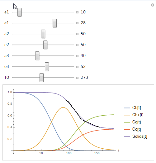
In your previous question posted here, the article you referenced spoke of ThermoGravimetric Analysis (TGA). If your data are also are derived from TGA, then the observable should be the total mass of solids remaining versus just $C_{B+}$. So, if you define $solids(t)$ as

$$solids(t)=C_{B}(t) + C_{B+}(t)+C_{C}(t)$$

You can obtain a much better fit with Manipulate because now the solids should asymptotically approach the fixed carbon or char level versus tend towards zero, which $C_{B+}$ does.

Here is the Manipulate with total solids included.

Manipulate[global = {a1, e1, a2, e2, a3, e3, T0}; 
 Show[Plot[
   Evaluate@({#[[1]][t], #[[2]][t], #[[3]][t], #[[4]][
         t], #[[1]][t] + #[[2]][t] + #[[4]][t]} &[
      sol[a1, e1, a2, e2, a3, e3, T0]]), {t, 0, 180}, 
   PlotLegends -> {"Cb[t]", "Cb+[t]", "Cg[t]", "Cc[t]", "Solids[t]"}, 
   AxesLabel -> Automatic], 
  ListPlot[data, PlotStyle -> {PointSize[Small], Black}]], {{a1, 
   10}, .5, 100, Appearance -> "Labeled"}, {{e1, 28}, 0, 40, 
  Appearance -> "Labeled"}, {{a2, 50}, 0, 100, 
  Appearance -> "Labeled"}, {{e2, 50}, 15, 80, 
  Appearance -> "Labeled"}, {{a3, 40}, 0, 100, 
  Appearance -> "Labeled"}, {{e3, 52}, 15, 80, 
  Appearance -> "Labeled"}, {{T0, 273}, 230, 320, 
  Appearance -> "Labeled"}]
Dynamic@global

Total Solids TGA

(* Dynamic@global = {10, 28, 50, 50, 40, 52, 273} *)

As with all chemical kinetic studies, it is desirable to have good initial and asymptotic data. A longer term study would tell you if the asymptote is zero or not.

Fit

We can create a model of the sum of solids from the parametric solution as shown

model[a1_, e1_, a2_, e2_, a3_, e3_, T0_][
   t_] := (#[[1]] + #[[2]] + #[[4]]) &@
    Through[sol[a1, e1, a2, e2, a3, e3, T0][t], List] /; 
   And @@ NumericQ /@ {a1, e1, a2, e2, a3, e3, T0};

We can create initial guesses using the dynamic global variable from our manipulate to populate a FindFit[] function like so

 initguess = 
 MapThread[List, {{a1, e1, a2, e2, a3, e3, T0}, First@Dynamic@global}]
fit = FindFit[data, model[a1, e1, a2, e2, a3, e3, T0][t], initguess, 
  t, Method -> "QuasiNewton"]
(* {a1 -> 9.99623, e1 -> 28.0077, a2 -> 49.9986, e2 -> 50.0113, 
 a3 -> 40.0015, e3 -> 51.9913, T0 -> 272.999} *)

The fit returned is very close to our initial guess.

It is doubtful that we will obtain unique fits. The data provided almost looks like two intersecting lines (needs 4 parameters to specify) and we are fitting 7 parameters. If you start from a worse initial guess and/or use different Methods, then you can obtain different parameter estimates.

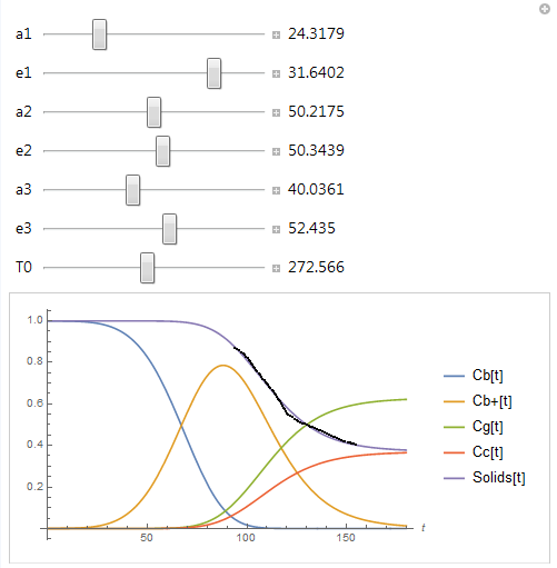
For example, if we start from a worse initial estimate and use the "ConjugateGradient" method, we still obtain a pretty good fit to the data as can be seen when the values are plugged into Manipulate.

fit = FindFit[data, 
  model[a1, e1, a2, e2, a3, e3, T0][
   t], {{a1, 25}, {e1, 28}, {a2, 50}, {e2, 50}, {a3, 40}, {e3, 
    52}, {T0, 273}}, t, Method -> "ConjugateGradient"]
(* {a1 -> 24.3179, e1 -> 31.6402, a2 -> 50.2175, e2 -> 50.3439, 
 a3 -> 40.0361, e3 -> 52.435, T0 -> 272.566} *)

Alternative Fit

$\endgroup$
2
  • $\begingroup$ Tim, I cannot express how grateful I am that you took the time to help me with this. You've made a more appropriate initial assumption! I was assuming that the intermediate was already formed in the TGA data Cb+ (I excluded the dehydration stage and secondary stage in the data I presented here). I'm a little out of my wheelhouse here, so thank you very much for helping me out. You've really gone the extra mile. I'll post an update with the rest of the data that explains the ending characteristics of the experiment. $\endgroup$ Commented May 10, 2019 at 17:43
  • $\begingroup$ @user3741793 Thank you for the kind words. I am glad it helped. I had some experience in a past life working on biomass gasification that gave me some insights to the problem. There is a lot of natural variation in biomass, which can make getting good data difficult. Best of luck! $\endgroup$
    – Tim Laska
    Commented May 10, 2019 at 22:51
1
$\begingroup$

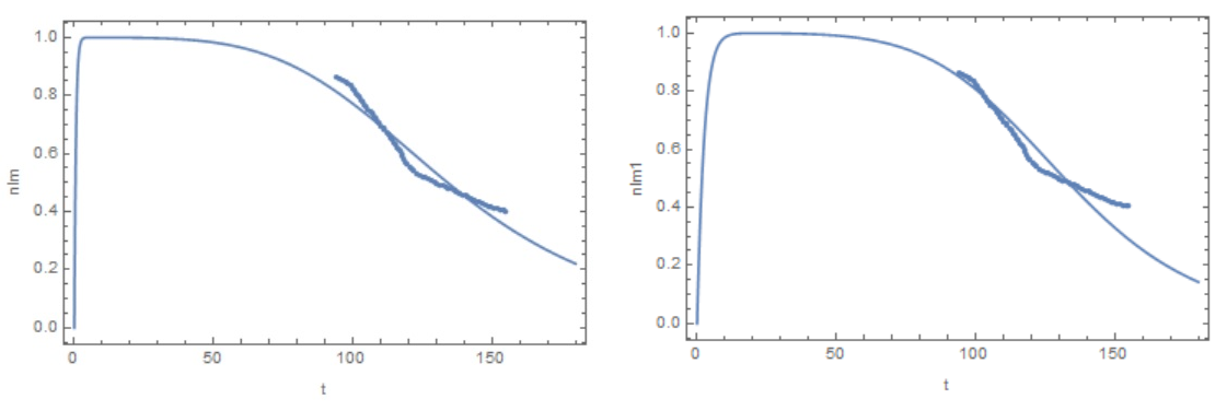
I found a working model. But parameter a3 turned out to be negative (nlm).Therefore, a second model has been created (nlm1).

data = {{94.30210177`, 0.864346486`}, {95.32514753`, 
    0.859754108`}, {96.34819329`, 0.854044984`}, {97.37123904`, 
    0.847107439`}, {98.30903099`, 0.839836015`}, {99.16156912`, 
    0.83232005`}, {99.92885344`, 0.823816908`}, {100.6108839`, 
    0.816520995`}, {101.2929145`, 0.808806302`}, {101.974945`, 
    0.800254051`}, {102.5717216`, 0.793411563`}, {103.1684983`, 
    0.784240661`}, {103.765275`, 0.77655503`}, {104.3620517`, 
    0.768897318`}, {104.9588284`, 0.760681234`}, {105.5556051`, 
    0.752716417`}, {106.2376356`, 0.744917968`}, {106.9196661`, 
    0.736365717`}, {107.6016966`, 0.727980977`}, {108.2837271`, 
    0.719428725`}, {108.9657576`, 0.711211497`}, {109.733042`, 
    0.702269474`}, {110.3298186`, 0.694721203`}, {111.0409556`, 
    0.687875903`}, {111.41376`, 0.680476135`}, {112.2054025`, 
    0.672472809`}, {112.9726869`, 0.664086925`}, {113.6547174`, 
    0.655255487`}, {114.1662402`, 0.648548153`}, {114.7630169`, 
    0.639606183`}, {115.3597936`, 0.63032919`}, {115.9736211`, 
    0.622771757`}, {116.485144`, 0.614992346`}, {116.9284638`, 
    0.60721385`}, {117.491139`, 0.598194166`}, {117.9856111`, 
    0.589510421`}, {118.5312355`, 0.580256448`}, {119.0257076`, 
    0.570534129`}, {119.7077381`, 0.561144318`}, {120.3897686`, 
    0.553429626`}, {121.1570529`, 0.545914804`}, {122.0948449`, 
    0.53833069`}, {123.1178906`, 0.532286543`}, {124.1409364`, 
    0.526689093`}, {125.1639821`, 0.520979969`}, {126.1870279`, 
    0.515829218`}, {127.2100737`, 0.510343443`}, {128.2331194`, 
    0.504745993`}, {129.2561652`, 0.500153615`}, {130.2792109`, 
    0.496231284`}, {131.3022567`, 0.492197279`}, {132.3253024`, 
    0.487939924`}, {133.3483482`, 0.484240942`}, {134.371394`, 
    0.480095262`}, {135.3944397`, 0.476284606`}, {136.4174855`, 
    0.473032322`}, {137.389379`, 0.469445701`}, {138.463577`, 
    0.463735891`}, {139.4866228`, 0.458808489`}, {140.5096685`, 
    0.454327785`}, {141.5327143`, 0.449735406`}, {142.55576`, 
    0.445366377`}, {143.5788058`, 0.440997348`}, {144.6018515`, 
    0.436069946`}, {145.6248973`, 0.431477568`}, {146.6479431`, 
    0.42666184`}, {147.6709888`, 0.421957787`}, {148.6940346`, 
    0.417700432`}, {149.5749906`, 0.414785078`}, {150.9106337`, 
    0.411863626`}, {151.9336795`, 0.409951437`}, {152.9567252`, 
    0.407257526`}, {153.979771`, 0.40467529`}, {155.0028168`, 
    0.402539752`}};

Rg = 8.314*10^-3;HR = 5;
n1 = 1;
n2 = 1.5;
n3 = 1.5;
model[a1_?NumberQ, e1_?NumberQ, a2_?NumberQ, e2_?NumberQ, a3_?NumberQ,
   e3_?NumberQ, T0_?NumberQ] :=  
 Module[{Cbp, x}, 
  First[Cbp /. 
    NDSolve[{Cb'[t] == -a1*E^(-e1/(Rg*T))*(Cb[t]^n1), 
       Cbp'[t] == 
        a1*E^(-e1/(Rg*T))*(Cb[t]^n1) - a2*E^(-e2/(Rg*T))*(Cbp[t]^n2) -
          a3*E^(-e3/(Rg*T))*(Cbp[t]^n3), 
       Cg'[t] == a2*E^(-e2/(Rg*T))*Cbp[t]^n2, 
       Cc'[t] == a3*E^(-e3/(Rg*T))*Cbp[t]^n3, Cb[0] == 1, Cbp[0] == 0,
        Cg[0] == 0, Cc[0] == 0} /. {T -> HR*t + T0}, {Cb, Cbp, Cg, 
      Cc}, {t, 0, 180}]]]

nlm = NonlinearModelFit[data, 
  model[a1, e1, a2, e2, a3, e3, T0][
   t], {{a1, 1.85}, {e1, 2.35}, {a2, 4.15}, {e2, 41.9}, {a3, 
    5.13}, {e3, 45.3}, {T0, 290}}, t, Method -> "Gradient"]
nlm["BestFitParameters"]

(*Out[]= {a1 -> 4.52721, e1 -> 2.31303, a2 -> 1.99788, e2 -> 32.0984, 
 a3 -> -2.61367, e3 -> 41.8827, T0 -> 291.747}*)

Fix some parameters including a3=4

nlm1 = 
 NonlinearModelFit[data, 
  model[a1, 2.31303, a2, 32.0986, 4, 41.8827, 291.747][t], {a1, a2}, 
  t, Method -> "Gradient"]

 nlm1["BestFitParameters"]

(*Out[]= {a1 -> 1.01459, a2 -> 0.507731}*)
{Show[Plot[nlm[t], {t, 0, 180}, PlotRange -> All], ListPlot[data], 
 Frame -> True, FrameLabel -> {"t", "nlm"}],Show[Plot[nlm1[t], {t, 0, 180}, PlotRange -> All], ListPlot[data], 
 Frame -> True, FrameLabel -> {"t", "nlm1"}]}

fig1

$\endgroup$
2
  • $\begingroup$ Hi Alex, Thank you very much for your valuable insight. With your help, I was able to get a much better fit to my data and understand how I could implement this again in the future. Tim (above) has corrected some flawed assumptions I had on the fit to begin with, which would have made your job probably much easier to begin with. You guys are both awesome and I truly appreciate your help! $\endgroup$ Commented May 10, 2019 at 16:33
  • $\begingroup$ @user3741793 You're welcome! Although I see that my code was useless due to an error in the model. $\endgroup$ Commented May 10, 2019 at 16:46

Your Answer

By clicking “Post Your Answer”, you agree to our terms of service and acknowledge you have read our privacy policy.

Not the answer you're looking for? Browse other questions tagged or ask your own question.