0
$\begingroup$

I have been experiencing very slow performance of NonlinearModelFit. The code that in my case causes that is below. The first part gets the data, the model and constraints and initial values. This is because, I have huge amount of functions combined.

ClearAll[cdata, fmodel, fitparmsconstr, fitparmsinit];
{cdata, fmodel, fitparmsconstr, fitparmsinit} = 
 CloudGet[
  "https://www.wolframcloud.com/obj/923620ca-ec70-43e3-b0f2-\
5f9311e14625"]

And now this takes insane amount of time, note that even with a single iteration, which should be immediate, it takes about two minutes.

NonlinearModelFit[cdata, {fmodel, fitparmsconstr}, fitparmsinit, x, 
 MaxIterations -> 1]

I realise that I have large amount of parameters, but when I did this model in FiTyk, it take 2 seconds to converge. I suspect there is some detail mathematica that i am missing. I cannot believe that with a single iteration it would be this bad.

(I am on Ma Linux 13.3.1.0)

Update on the purpose.

The data come from coupled mass spectroscopy (MS) with thermogravometric analysis (TGA). The problem with TGA is that when you compute the mass loss derivative (DTG curve), it has many peaks which are superimposed onto each other and impossible to resolve which peak is from what species or in other words how much of what species was lost. However, I do have data from mass spectroscopy for each chemical species so I know for say water, the peaks, where they occur and how wide they are. Those I fitted in FiTyk. And so for water, i have a sum of n1 gaussians, for CO2 I have sum of n2 gaussians etc.

Now come some assumptions (don't stone me for them). Basic assumption is that the peaks on MS are also gaussians. Next, I assume that when peak is observed in MS data, there should be a peak in the DTG (this is quite valid as the molecules in the system travel fast compared to the measure time), nevertheless there might be a bit of an offset between the peaks from MS to DTG data but this offset should be the same for each species (thus the first set of free parameters called \[Delta]c with number denoting a specific species). Second assumption is that I do not know the peak heights in DTG data but the peaks should keep proportional, that is if peak 1 was twice as high as peak 2 for a particular specie, this relationship should be preserved, that gives another set of free parameters \[Delta]h. Finally, the assumption is that the peaks should be more or less the same width, there can be some dispersion and the freedom for that constitutes the last set of parameters \[Delta]w.

Now constraints are formed because even Fityk tends to fit the data with negative peaks or because the peaks tend to shift unreasonably too much.

$\endgroup$

2 Answers 2

3
$\begingroup$

You didn't show your results but your code provides poor results on my machine.

$Version

(* "14.0.0 for Mac OS X ARM (64-bit) (December 13, 2023)" *)

Clear["Global`*"]

{cdata, fmodel, fitparmsconstr, fitparmsinit} = 
  CloudGet["https://www.wolframcloud.com/obj/923620ca-ec70-43e3-b0f2-\
5f9311e14625"];

{xmin, xmax} = MinMax[cdata[[All, 1]]];

(nlm = NonlinearModelFit[cdata, {fmodel, fitparmsconstr}, fitparmsinit, x];) //
 AbsoluteTiming

(* {42.1485, Null} *)

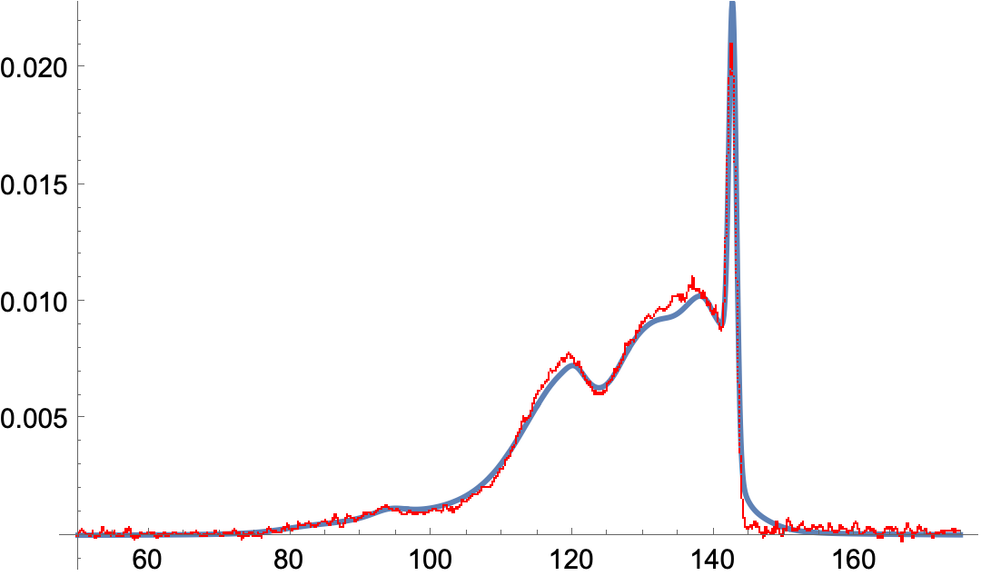
The fit is very poor.

Show[
  Plot[nlm[x], {x, xmin, xmax},
   PlotPoints -> 50,
   MaxRecursion -> 5,
   PlotRange -> {Automatic, 0.025}],
  ListPlot[cdata, PlotStyle -> Red]] //
 Quiet

enter image description here

Using Method -> "NMinimize"

(sys = Simplify[Rationalize[
     {cdata, {fmodel, fitparmsconstr}, fitparmsinit, x, 
      Method -> "NMinimize"}, 0]]);

Much slower

(nlm2 = NonlinearModelFit @@ sys;) // AbsoluteTiming

(* {138.283, Null} *)

But a much improved fit.

Show[
  Plot[nlm2[x], {x, xmin, xmax},
   PlotPoints -> 50,
   MaxRecursion -> 5,
   PlotRange -> {Automatic, 0.025}],
  ListPlot[cdata, PlotStyle -> Red],
  PlotRange -> All] // Quiet

enter image description here

$\endgroup$
3
$\begingroup$

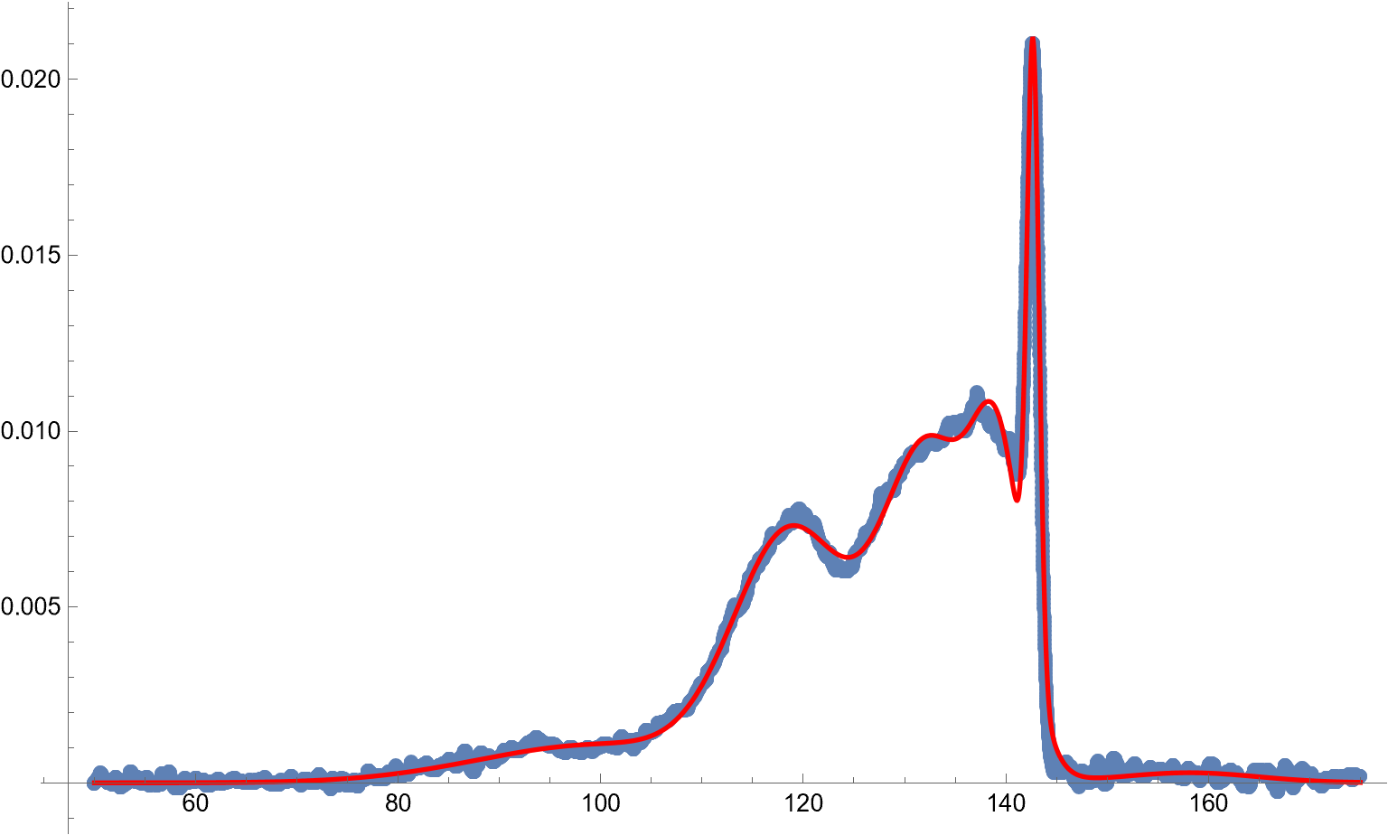
Your model is a bit "different" in that it is not the sum of 6 separate Gaussian-shaped functions. If you did use 6 separate Gaussian-shaped functions, you could get a better fit and much quicker. The quickness seems mostly dependent on reasonable starting values for the centers of those functions.

{cdata, fmodel, fitparmsconstr, fitparmsinit} = CloudGet[
   "https://www.wolframcloud.com/obj/923620ca-ec70-43e3-b0f2-5f9311e14625"];
{xmin, xmax} = MinMax[cdata[[All, 1]]];

model = Sum[α[i] Exp[-(x - μ[i])^2/(2 σ[i]^2)], {i, 1, 6}];
parms = {α[1], α[2], α[3], α[4], α[5], α[6],
         σ[1], σ[2], σ[3], σ[4], σ[5], σ[6],
         {μ[1], 95}, {μ[2], 119}, {μ[3], 130}, {μ[4], 137}, {μ[5], 143}, {μ[6], 160}};
(nlm = NonlinearModelFit[cdata, model, parms, x, MaxIterations -> 1000] // Quiet) // AbsoluteTiming
Show[ListPlot[cdata, PlotStyle -> PointSize[0.01], ImageSize -> Large], 
  Plot[nlm[x], {x, xmin, xmax}, PlotStyle -> Red]] // Quiet

Plot of data and fit

Your model looks like it is constructed as some other fit (like maybe from a journal article) with the parameters being the deviations you believe exist from that journal article. In any event, it would be helpful for you to describe why your model looks the way it does.

Addition

If the construction of your model makes sense (and I'm not saying it doesn't - I'm just saying that I don't know the subject matter but I'm initially skeptical of the construction which throws in estimates for other analyses as if those were estimated without error), then using a small fraction of the data points to get initial estimates results in a much better and faster fit. (Good starting values are your best friends.)

{cdata, fmodel, fitparmsconstr, fitparmsinit} = 
  CloudGet["https://www.wolframcloud.com/obj/923620ca-ec70-43e3-b0f2-5f9311e14625"];

{xmin, xmax} = MinMax[cdata[[All, 1]]];

(* Fit with 1/20th of the number of data points *)
cdata20 = cdata[[Range[1, Length[cdata], 20]]];
(sys = Simplify[Rationalize[{cdata20, {fmodel, fitparmsconstr}, fitparmsinit, x,
   Method -> "NMinimize"}, 0]]);
(nlm2 = NonlinearModelFit @@ sys;) // AbsoluteTiming
(* {113.097, Null} *)

(* Use all data and previous fit as starting values *)
fitparmsinit = # /. Rule -> List & /@ nlm2["BestFitParameters"]
sys = {cdata, {fmodel, fitparmsconstr}, fitparmsinit, x};
(nlm3 = NonlinearModelFit @@ sys;) // AbsoluteTiming
(* {184.296, Null} *)

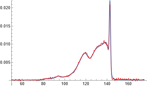
Show[Plot[nlm3[x], {x, xmin, xmax}],
  ListPlot[cdata, PlotStyle -> Red], PlotRange -> All] // Quiet

Data and fit with original model

Good starting values are needed in part because there are several extreme correlations among the parameter estimators (such as -0.999898 and +0.99874). That can confuse most iterative procedures looking for a maximum (or minimum) function value.

$\endgroup$
2
  • $\begingroup$ I added an explanation of the model. Can you please elaborate on what you mean by "sum of 6 separate Gaussian-shaped functions"? $\endgroup$
    – atapaka
    Commented Apr 3 at 13:22
  • $\begingroup$ Thanks. That helps. So what I produced simply gives a reasonable reproduction of cdata without any ability to sort out contributions from each species. Is the reproduction of the cdata the objective or is it essential to sort out the individual species contributions? $\endgroup$
    – JimB
    Commented Apr 3 at 17:15

Your Answer

By clicking “Post Your Answer”, you agree to our terms of service and acknowledge you have read our privacy policy.

Not the answer you're looking for? Browse other questions tagged or ask your own question.