replaced http://mathematica.stackexchange.com/ with https://mathematica.stackexchange.com/
Source Link

It seems it is better to use a family of functions instead of just one. The code below uses NonLinearFit instead of FindFit, since I do not think using FindFit is a hard requirement in the question.

Also, below I assume that the definitions in the question are evaluated.

First, let us speed-up the use of NIntegrate:

T[(beta_)?NumericQ, (Is_)?NumericQ, (z_)?NumericQ] := 
  Q[z, Is]/(Sqrt[Pi]*q[z, beta])*
   NIntegrate[
    Log[1 + q[z, beta]*Exp[-t^2]], {t, -\[Infinity], \[Infinity]}, 
    PrecisionGoal -> 3, 
    Method -> {Automatic, "SymbolicProcessing" -> 0}];

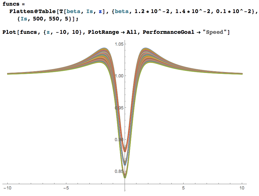
Second, let us select and plot a family of functions:

funcs = Flatten@
   Table[T[beta, Is, z], {beta, 1.2*10^-2, 1.4*10^-2, 0.1*10^-2}, {Is, 500, 550, 5}];

Plot[funcs, {z, -10, 10}, PlotRange -> All, 
 PerformanceGoal -> "Speed"]

enter image description here

(I selected the functions using the ranges of the parameters given to FindFit in the question.)

Next we create linear combinations variables:

vars = Array[a, Length[funcs]];

...and do a model fit:

fm = NonlinearModelFit[data, vars.funcs, vars, z, 
  Method -> "NMinimize"]

Notice the choice of the method. With the default method I was getting singular curves (which were still providing a good fit).

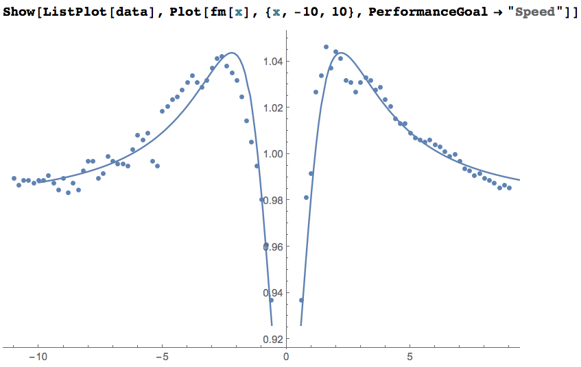
Finally, we plot the data and the model function:

Show[ListPlot[data], 
 Plot[fm[x], {x, -10, 10}, PerformanceGoal -> "Speed"]]

enter image description here

This question and my response are very similar to Non-linear curve fit problemNon-linear curve fit problem.

It seems it is better to use a family of functions instead of just one. The code below uses NonLinearFit instead of FindFit, since I do not think using FindFit is a hard requirement in the question.

Also, below I assume that the definitions in the question are evaluated.

First, let us speed-up the use of NIntegrate:

T[(beta_)?NumericQ, (Is_)?NumericQ, (z_)?NumericQ] := 
  Q[z, Is]/(Sqrt[Pi]*q[z, beta])*
   NIntegrate[
    Log[1 + q[z, beta]*Exp[-t^2]], {t, -\[Infinity], \[Infinity]}, 
    PrecisionGoal -> 3, 
    Method -> {Automatic, "SymbolicProcessing" -> 0}];

Second, let us select and plot a family of functions:

funcs = Flatten@
   Table[T[beta, Is, z], {beta, 1.2*10^-2, 1.4*10^-2, 0.1*10^-2}, {Is, 500, 550, 5}];

Plot[funcs, {z, -10, 10}, PlotRange -> All, 
 PerformanceGoal -> "Speed"]

enter image description here

(I selected the functions using the ranges of the parameters given to FindFit in the question.)

Next we create linear combinations variables:

vars = Array[a, Length[funcs]];

...and do a model fit:

fm = NonlinearModelFit[data, vars.funcs, vars, z, 
  Method -> "NMinimize"]

Notice the choice of the method. With the default method I was getting singular curves (which were still providing a good fit).

Finally, we plot the data and the model function:

Show[ListPlot[data], 
 Plot[fm[x], {x, -10, 10}, PerformanceGoal -> "Speed"]]

enter image description here

This question and my response are very similar to Non-linear curve fit problem.

added 1 character in body
Source Link
Anton Antonov
  • 38k
  • 3
  • 103
  • 179

It seems it is better to use a family of functions instead of just one. The code below uses NonLinearFit instead of FindFit, since I do not think using FindFit is a hard requirement in the question.

Also, below I assume that the definitions in the question are evaluated.

First, let us speed-up the use of NIntegrate:

T[(beta_)?NumericQ, (Is_)?NumericQ, (z_)?NumericQ] := 
  Q[z, Is]/(Sqrt[Pi]*q[z, beta])*
   NIntegrate[
    Log[1 + q[z, beta]*Exp[-t^2]], {t, -\[Infinity], \[Infinity]}, 
    PrecisionGoal -> 3, 
    Method -> {Automatic, "SymbolicProcessing" -> 0}];

Second, let us select and plot a family of functions:

funcs = Flatten@
   Table[T[beta, Is, z], {beta, 1.2*10^-2, 1.4*10^-2, 0.1*10^-2}, {Is, 500, 550, 5}];

Plot[funcs, {z, -10, 10}, PlotRange -> All, 
 PerformanceGoal -> "Speed"]

enter image description here

(I selected the functions using the ranges of the parameters given to FindFit in the question.)

Next we create linear combinations variables:

vars = Array[a, Length[funcs]];

...and do a model fit:

fm = NonlinearModelFit[data, vars.funcs, vars, z, 
  Method -> "Minimize"]"NMinimize"]

Notice the choice of the method. With the default method I was getting singular curves (which were still providing a good fit).

Finally, we plot the data and the model function:

Show[ListPlot[data], 
 Plot[fm[x], {x, -10, 10}, PerformanceGoal -> "Speed"]]

enter image description here

This question and my response are very similar to Non-linear curve fit problem.

It seems it is better to use a family of functions instead of just one. The code below uses NonLinearFit instead of FindFit, since I do not think using FindFit is a hard requirement in the question.

Also, below I assume that the definitions in the question are evaluated.

First, let us speed-up the use of NIntegrate:

T[(beta_)?NumericQ, (Is_)?NumericQ, (z_)?NumericQ] := 
  Q[z, Is]/(Sqrt[Pi]*q[z, beta])*
   NIntegrate[
    Log[1 + q[z, beta]*Exp[-t^2]], {t, -\[Infinity], \[Infinity]}, 
    PrecisionGoal -> 3, 
    Method -> {Automatic, "SymbolicProcessing" -> 0}];

Second, let us select and plot a family of functions:

funcs = Flatten@
   Table[T[beta, Is, z], {beta, 1.2*10^-2, 1.4*10^-2, 0.1*10^-2}, {Is, 500, 550, 5}];

Plot[funcs, {z, -10, 10}, PlotRange -> All, 
 PerformanceGoal -> "Speed"]

enter image description here

(I selected the functions using the ranges of the parameters given to FindFit in the question.)

Next we create linear combinations variables:

vars = Array[a, Length[funcs]];

...and do a model fit:

fm = NonlinearModelFit[data, vars.funcs, vars, z, 
  Method -> "Minimize"]

Notice the choice of the method. With the default method I was getting singular curves (which were still providing a good fit).

Finally, we plot the data and the model function:

Show[ListPlot[data], 
 Plot[fm[x], {x, -10, 10}, PerformanceGoal -> "Speed"]]

enter image description here

This question and my response are very similar to Non-linear curve fit problem.

It seems it is better to use a family of functions instead of just one. The code below uses NonLinearFit instead of FindFit, since I do not think using FindFit is a hard requirement in the question.

Also, below I assume that the definitions in the question are evaluated.

First, let us speed-up the use of NIntegrate:

T[(beta_)?NumericQ, (Is_)?NumericQ, (z_)?NumericQ] := 
  Q[z, Is]/(Sqrt[Pi]*q[z, beta])*
   NIntegrate[
    Log[1 + q[z, beta]*Exp[-t^2]], {t, -\[Infinity], \[Infinity]}, 
    PrecisionGoal -> 3, 
    Method -> {Automatic, "SymbolicProcessing" -> 0}];

Second, let us select and plot a family of functions:

funcs = Flatten@
   Table[T[beta, Is, z], {beta, 1.2*10^-2, 1.4*10^-2, 0.1*10^-2}, {Is, 500, 550, 5}];

Plot[funcs, {z, -10, 10}, PlotRange -> All, 
 PerformanceGoal -> "Speed"]

enter image description here

(I selected the functions using the ranges of the parameters given to FindFit in the question.)

Next we create linear combinations variables:

vars = Array[a, Length[funcs]];

...and do a model fit:

fm = NonlinearModelFit[data, vars.funcs, vars, z, 
  Method -> "NMinimize"]

Notice the choice of the method. With the default method I was getting singular curves (which were still providing a good fit).

Finally, we plot the data and the model function:

Show[ListPlot[data], 
 Plot[fm[x], {x, -10, 10}, PerformanceGoal -> "Speed"]]

enter image description here

This question and my response are very similar to Non-linear curve fit problem.

Better grammar.
Source Link
Anton Antonov
  • 38k
  • 3
  • 103
  • 179

It seems it is better to use a family of functions instead of just one. The code below useuses NonLinearFit instead of FindFit, since I do not think using FindFit is a hard requirement in the question.

Also, below I assume that the definitions in the questionsquestion are evaluated.

First, let us speed-up the use of NIntegrate:

T[(beta_)?NumericQ, (Is_)?NumericQ, (z_)?NumericQ] := 
  Q[z, Is]/(Sqrt[Pi]*q[z, beta])*
   NIntegrate[
    Log[1 + q[z, beta]*Exp[-t^2]], {t, -\[Infinity], \[Infinity]}, 
    PrecisionGoal -> 3, 
    Method -> {Automatic, "SymbolicProcessing" -> 0}];

Second, let useus select and plot a family of functions:

funcs = Flatten@
   Table[T[beta, Is, z], {beta, 1.2*10^-2, 1.4*10^-2, 0.1*10^-2}, {Is, 500, 550, 5}];

Plot[funcs, {z, -10, 10}, PlotRange -> All, 
 PerformanceGoal -> "Speed"]

enter image description here

(I selected the functions using the ranges of the parameters given to FindFit in the question.)

Next we create linear combinations variables:

vars = Array[a, Length[funcs]];

...and do a model fit:

fm = NonlinearModelFit[data, vars.funcs, vars, z, 
  Method -> "Minimize"]

Notice the choice of the method. With the default method I was getting singular curves (which were still providing a good fit).

Finally, we plot the model functiondata and the datamodel function:

Show[ListPlot[data], 
 Plot[fm[x], {x, -10, 10}, PerformanceGoal -> "Speed"]]

enter image description here

This question and my response are very similar to Non-linear curve fit problem.

It seems it is better to use a family of functions instead of just one. The code below use NonLinearFit instead of FindFit, since I do not think using FindFit is a hard requirement in the question.

Also, below I assume that the definitions in the questions are evaluated.

First, let us speed-up the use of NIntegrate:

T[(beta_)?NumericQ, (Is_)?NumericQ, (z_)?NumericQ] := 
  Q[z, Is]/(Sqrt[Pi]*q[z, beta])*
   NIntegrate[
    Log[1 + q[z, beta]*Exp[-t^2]], {t, -\[Infinity], \[Infinity]}, 
    PrecisionGoal -> 3, 
    Method -> {Automatic, "SymbolicProcessing" -> 0}];

Second, let use select and plot a family of functions:

funcs = Flatten@
   Table[T[beta, Is, z], {beta, 1.2*10^-2, 1.4*10^-2, 0.1*10^-2}, {Is, 500, 550, 5}];

Plot[funcs, {z, -10, 10}, PlotRange -> All, 
 PerformanceGoal -> "Speed"]

enter image description here

(I selected the functions using the ranges of the parameters given to FindFit in the question.)

Next we create linear combinations variables:

vars = Array[a, Length[funcs]];

...and do a model fit:

fm = NonlinearModelFit[data, vars.funcs, vars, z, 
  Method -> "Minimize"]

Notice the choice of the method. With the default method I was getting singular curves (which were still providing a good fit).

Finally, we plot the model function and the data:

Show[ListPlot[data], 
 Plot[fm[x], {x, -10, 10}, PerformanceGoal -> "Speed"]]

enter image description here

This question and my response are very similar to Non-linear curve fit problem.

It seems it is better to use a family of functions instead of just one. The code below uses NonLinearFit instead of FindFit, since I do not think using FindFit is a hard requirement in the question.

Also, below I assume that the definitions in the question are evaluated.

First, let us speed-up the use of NIntegrate:

T[(beta_)?NumericQ, (Is_)?NumericQ, (z_)?NumericQ] := 
  Q[z, Is]/(Sqrt[Pi]*q[z, beta])*
   NIntegrate[
    Log[1 + q[z, beta]*Exp[-t^2]], {t, -\[Infinity], \[Infinity]}, 
    PrecisionGoal -> 3, 
    Method -> {Automatic, "SymbolicProcessing" -> 0}];

Second, let us select and plot a family of functions:

funcs = Flatten@
   Table[T[beta, Is, z], {beta, 1.2*10^-2, 1.4*10^-2, 0.1*10^-2}, {Is, 500, 550, 5}];

Plot[funcs, {z, -10, 10}, PlotRange -> All, 
 PerformanceGoal -> "Speed"]

enter image description here

(I selected the functions using the ranges of the parameters given to FindFit in the question.)

Next we create linear combinations variables:

vars = Array[a, Length[funcs]];

...and do a model fit:

fm = NonlinearModelFit[data, vars.funcs, vars, z, 
  Method -> "Minimize"]

Notice the choice of the method. With the default method I was getting singular curves (which were still providing a good fit).

Finally, we plot the data and the model function:

Show[ListPlot[data], 
 Plot[fm[x], {x, -10, 10}, PerformanceGoal -> "Speed"]]

enter image description here

This question and my response are very similar to Non-linear curve fit problem.

Source Link
Anton Antonov
  • 38k
  • 3
  • 103
  • 179
Loading