Calling Correct Function for Plotting DiracDelta

Question

I am wondering what is the correct function in Mathematica to plot the true impulse function, better known as the DiracDelta[] function. When using this inside of a function or just the function itself when plotting, it renders output = zero. Quick example:

Plot[DiracDelta[x], {x,-1,1}]

I am wondering, is this the correct delta function which is infinite in height at zero and zero everywhere else. I have seen other functions such as KroneckerDelta[], but this seems to do the same exact thing. The code is below:

eqn1wb := (2 ((I Pi f) Exp[(-I) 2 Pi f]) ((1/2) DiracDelta[f-2] + 
          DiracDelta[f+2]))/(1 + I 2 Pi f); 
wb1 = Plot[Re[eqn1wb], {f, -5, 5}, 
PlotRange :> All, PlotStyle :> {Thick, Red},
AspectRatio :> 1,
GridLines :> {{-4, -2, 2, 4}, {1.0, 0.5, -0.5, -1.0}}, 
PlotLabel :> "Re(w) - Frequency Response", 
AxesLabel :> {"f", "W(f)"}
]

Answer 1

To create the plot you could replace any occurrence of DiracDelta[a] with something like 10000 UnitStep[1/10000 - a^2]], so for example to plot

f[x_] := DiracDelta[x - 2] + DiracDelta[x + 2]

you could do something like

Plot[Evaluate[f[x] /. DiracDelta[a_] :> 10000 UnitStep[1/10000 - a^2]], 
  {x, -4, 4}, Exclusions -> None, PlotPoints -> 800]

Note that for Mathematica to see the discontinuities you need to increase the number of plot points. The number of points needed will depend on the plot range, so you might have to tweak that.

Answer 2

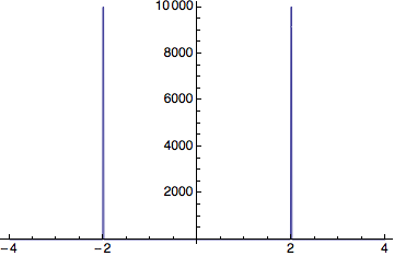
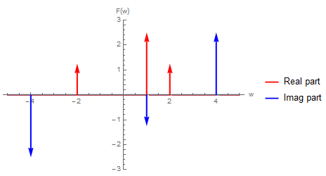
As others already have written, the Dirac delta is not a real function and it can't be plotted. Other programs that claim to plot it just fake it.

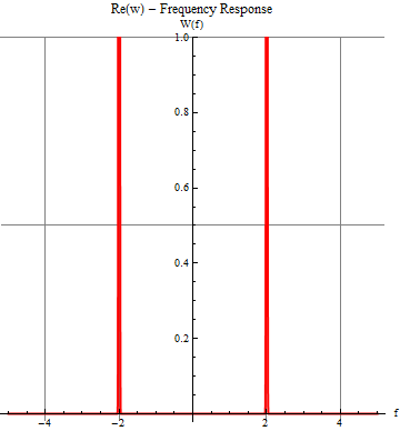
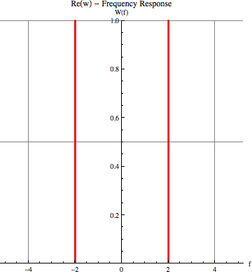
Having said that, you can roll a diracDelta of your own, that more or less mimics the Dirac Delta's behavior but is still continuous. Advantage with respect to Heike's solution is that we don't need to increase the number of PlotPoints. I'll use the NormalDistrution with a very small standard deviation:

diracDelta[x_] = PDF[NormalDistribution[0, 1/100], x];

eqn1wb := (2 ((I Pi f) Exp[(-I) 2 Pi f]) ((1/2) DiracDelta[f - 2] + 
       DiracDelta[f + 2]))/(1 + I 2 Pi f);

wb1 = Plot[
  Re[eqn1wb] /. DiracDelta -> diracDelta // Evaluate, {f, -5, 5}, 
  PlotStyle :> {Thick, Red}, AspectRatio :> 1, 
  GridLines :> {{-4, -2, 2, 4}, {1.0, 0.5, -0.5, -1.0}}, 
  PlotLabel :> "Re(w) - Frequency Response", 
  AxesLabel :> {"f", "W(f)"}, PlotRange -> {Automatic, 1.5}]

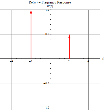
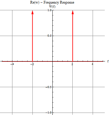
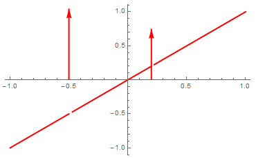
DiracDelta's are sometimes plotted by using arrows. Of course we can do that as well. In this case we can set the function at zero everywhere and add arraows in the Epilog part of the plot.

 Plot[0, {f, -5, 5}, PlotStyle :> {Thick, Red}, AspectRatio :> 1,
   GridLines :> {{-4, -2, 2, 4}, {1.0, 0.5, -0.5, -1.0}}, 
  PlotLabel :> "Re(w) - Frequency Response", 
  AxesLabel :> {"f", "W(f)"}, PlotRange -> {Automatic, 1.}, 
  Epilog -> {Red, Thick,Arrow[{{-2, 0}, {-2, 1}}], Arrow[{{2, 0}, {2, 1}}]}]

I believe the convention is to scale the lengths of the arrows in proportion to the factors in front of the DiracDelta. The above can be easily extended to do that.

Factors can be found using Coefficient:

Coefficient[eqn1wb, DiracDelta[-2 + f]]

(*
==> (I E^(-2 I f \[Pi]) f \[Pi])/(1 + 2 I f \[Pi])
*)

Ratio's of coefficients:

Coefficient[eqn1wb, DiracDelta[2 + f]]/Coefficient[eqn1wb, DiracDelta[2 - f]]

(*
==> 2
*)

Locations of the Dirac delta's:

Cases[eqn1wb, DiracDelta[a__] :> Solve[a == 0, f], Infinity]

(*
==> {{{f -> 2}}, {{f -> -2}}}
*)

I'm not going to automate it all, but the idea is clear. In the end you'll get something like:

Answer 3

The Dirac delta, $\delta(x)$ is zero everywhere except at zero, and has an integral of 1 over $\mathbb{R}$. It is not really a function in the true sense and equating $\delta(0)=\infty$ is a rather loose definition; it should technically be considered as a distribution or a delta measure. Mathematica's implementation of DiracDelta remains unevaluated at 0 and has all the other properties.

DiracDelta /@ {-1, 0, 1}
Out[1]= {0, DiracDelta[0], 0}

Integrate[DiracDelta[x] , {x, -Infinity, Infinity}]
Out[2]= 1

This explains why you weren't getting any result with Plot.

In the off-chance that you were trying to plot the impulse response of a discrete-time system, then you might be interested in the DiscreteDelta function:

ListPlot[DiscreteDelta /@ Range[-5, 5], Filling -> Axis, PlotMarkers -> {Automatic, 10}]

---

You can also reproduce your MATLAB "plot" of the Dirac delta function in Mathematica. Let me first note that you're not using their dirac() function to produce the output you've shown below. In fact, they define it "loosely":

function Y = dirac(X)
%DIRAC  Delta function.
%    DIRAC(X) is zero for all X, except X == 0 where it is infinite.
%    more comments

Y = zeros(size(X));
Y(X == 0) = Inf;

and this would not have given you the plot you showed, because of the Inf. You have probably replaced Inf with 10000 or written a similar function. Heike, image_doctor and Sjoerd have shown you ways of plotting it. You can also roll your own, a la MATLAB style as:

dirac[x_] := Piecewise[{{10000, x == 0}, {0, True}}]
ListLinePlot[{#, dirac@#} & /@ Range[-1, 1, 1/1000], Frame -> True, Axes -> False]

Now use this definition to redefine DiracDelta inside a Block and you can use your original code with some slight modifications:

wb1 = Block[{DiracDelta = Piecewise[{{10000, # == 0}, {0, True}}] &}, 
  ListLinePlot[Re[eqn1wb] /. f -> # & /@ Range[-5, 5, 1/100], 
   DataRange -> {-5, 5}, PlotRange :> {All, {0, 1}}, 
   PlotStyle :> {Thick, Red}, AspectRatio :> 1, 
   GridLines :> {{-4, -2, 2, 4}, {1.0, 0.5, -0.5, -1.0}}, 
   PlotLabel :> "Re(w) - Frequency Response", 
   AxesLabel :> {"f", "W(f)"}]
  ]

If I were to use a schematic to show the delta function, I would do it similar to Sjoerd's arrow plots.

Answer 4

Building on Sjoerd C. de Vries's solution, I wrote this little function to make the task easy for anyone interested in plotting Dirac's Delta as arrows in a Plot command in Mathematica. The function receives an equation and a variable, and returns a list of {Arrow[]}'s in the correct location of the Diract Deltas, that can be included in the Epilog of a Plot command.

ArrowsDeltaFunction[eqn_, x_] := Module[{xsubs, listDeltas, coefDeltas, locationDeltas},
  xsubs = (x /. Cases[eqn, DiracDelta[a__] :> Solve[a == 0, x], Infinity]) /. x -> {};
  listDeltas = DiracDelta[x - x0] /. x0 -> xsubs;
  coefDeltas = Flatten[Coefficient[eqn, listDeltas]];
  locationDeltas = Flatten[xsubs];

  Arrow[Table[{{locationDeltas[[i]], 0}, {locationDeltas[[i]], 
      coefDeltas[[i]]}}, {i, 1, Length[locationDeltas]}]]
]

So you can use this function throughout your code by including it in the Plot Epilog, like this:

eqn1 := x + (3/4) DiracDelta[x - 0.2] + (\[Pi]/3) DiracDelta[x + 0.5]

Plot[eqn1, {x, -5, 5},
   PlotStyle -> {Thick, Red},
   Epilog -> {Thick, Red, ArrowsDeltaFunction[eqn1, x]}
]

You can see the arrows appear in the "gaps" of the function where the Delta's exist, and their height correspond to the coefficient of the Delta. The code works even if the function does not have Deltas (no arrows are plotted).

Edit: This can have nice applications for teachers to explain Fourier Transforms, its properties, etc.

(* Time Domain Signal (in this case complex) *)
Ft :=  (1 - I/2) Exp[-I t] +  Cos[2 t]  + 2 Sin[4 t]

(* Fourier Transform *)
Fw := FourierTransform[Ft, t, w] 
ReFw := ComplexExpand[Re[Fw]]
ImFw := ComplexExpand[Im[Fw]]

(* Plot *)
Plot[{ReFw, ImFw}, {w, -5, 5},
 PlotStyle -> {Thick, Red, Blue},
 PlotRange -> 3,
 AxesLabel -> {"w", "F(w)"},
 PlotLegends -> LineLegend[{Red, Blue}, {"Real part", "Imag part"}],
 Epilog -> {Thick, 
    Red, ArrowsDeltaFunction[ReFw, w], 
    Blue, ArrowsDeltaFunction[ImFw, w] 
 }
]

Answer 5

At your own risk, you can redefine the DiracDelta function to have the behaviour you want:

Unprotect@DiracDelta;
DiracDelta[0] := your large number;
Protect@DiracDelta;

The integral given by

Integrate[DiracDelta[x], {x, -Infinity, Infinity}]

still seems to equate to one with the new definition in place.