Specific initial sample points for 3D plots

Question

PlotPoints lets you determine how many sample points you want in each direction, but sometimes I want specific ones.

For Plot you can give an argument like PlotPoints->{None, pts} to use pts as the initial points:

Show[
 Plot[Sin[x], {x, -3 Pi, 3 Pi},
  PlotStyle -> Red,
  MaxRecursion -> 0,
  PlotPoints -> {None, {-7.3, -5.2, -Pi, Pi, 3.8, 5}},
  PlotRange -> {{-3 Pi, 3 Pi}, {-1, 1}}],
 Plot[Sin[x], {x, -5 Pi, 5 Pi},PlotStyle -> Dashed]
 ]

Is this also possible for Plot3D? Whatever I try I end up with completely broken plots, anyone know the syntax of what I have stumbled into?

EDIT

PlotPoints->{Automatic,pts} seems to work, although about 2x as many points are used.

f[x_, y_] := Cos[y]^3 Sin[x]^2 + Cos[x] Sin[y]
pts3d = Reap[Plot3D[f[x, y], {x, -5, 5}, {y, -5, 5},
                    EvaluationMonitor :> Sow[{x, y}]]][[-1, 1]];
opts = {{Automatic, "Automatic"},
        {{None, pts3d}, "{None, pts3d}"},
        {{Automatic, pts3d}, "{Automatic,pts3d}"},
        {{Automatic, RandomReal[{-5, 5}, {5000, 2}]}, "{Automatic,Random}"}
        };
Row[Plot3D[f[x, y], {x, -5, 5}, {y, -5, 5},
    PlotPoints -> First@#,
    PlotLabel -> Last@#,
    ImageSize -> 200] & /@ opts]

Here are three plots with exactly the same points that look different:

{orig, {origpts}} = Reap[DensityPlot[f[x, y], {x, -5, 5}, {y, -5, 5},
    EvaluationMonitor :> Sow[{x, y}]]];
{auto, {autopts}} = Reap[DensityPlot[f[x, y], {x, -5, 5}, {y, -5, 5},
    PlotPoints -> {Automatic, RandomSample[origpts]},
    MaxRecursion -> 0,
    EvaluationMonitor :> Sow[{x, y}]]];
{none, {nonepts}} = Reap[DensityPlot[f[x, y], {x, -5, 5}, {y, -5, 5},
    PlotPoints -> {None, RandomSample[origpts]},
    MaxRecursion -> 0,
    EvaluationMonitor :> Sow[{x, y}]]];

(* All give {} *)
DeleteCases[origpts, Alternatives @@ autopts]
DeleteCases[autopts, Alternatives @@ origpts]
DeleteCases[nonepts, Alternatives @@ origpts]

{orig, auto, none}

Answer 1

Just to be clear, the following is based on experimentation and could be wildly misleading...

The outline of the algorithm for generating the mesh for Plot3D and DensityPlot appears to be:

• Create initial mesh based on the number of plot points
• Inject any user supplied points into the mesh
• Refine the mesh

There are two issues to worry about when supplying an explicit list of points to PlotPoints. The first is that the injection of a point into the initial mesh works by subdividing the containing triangle, which can lead to very long thin triangles in the mesh. The second, critical, issue is that the mesh refinement appears to fail if too many points are inserted into a coarse initial mesh.

To demonstrate these issues I will define a function to show the mesh obtained with specified PlotPoints and MaxRecursion settings:

showmesh[pp_, mr_, opts___] :=
 DensityPlot[f[x, y], {x, -1, 1}, {y, -1, 1},
  Mesh -> All, MeshStyle -> Red, ColorFunction -> (White &),
  Frame -> None,
  PlotPoints -> pp, MaxRecursion -> mr, opts]

f[x_, y_] := 1

To start with we can look at the mesh obtained with no refinement and a small number of plot points. There are no surprises here:

GraphicsRow[showmesh[#, 0] & /@ {2, 3, 4}]

When an explicit extra point is supplied, the containing triangle is subdivided:

p = {{-0.123, 0.123}};   
GraphicsRow[showmesh[{#, p}, 0] & /@ {2, 3, 4}]

The thin triangle issue is clear, compare for example the first mesh above with a Delaunay triangulation of the same points:

If we allow some mesh refinement with MaxRecursion, we can see that the user specified point is sampled after the initial mesh points but before the refinement. I've highlighted the user specified point in red:

Reap[showmesh[{3, p}, 3, EvaluationMonitor :> Sow[{x, y}]]][[2]] /. x : First[p] :> Style[x, Red]

I'll now switch to a more interesting plot function to make the refinement more obvious. Here are the meshes with our single user-specified point and adaptive mesh refinement switched on:

f[x_, y_] := Sin[20 x y]    
GraphicsRow[showmesh[{#, p}, 3] & /@ {2, 3, 4}]

Something interesting has happened - the meshes with 3 and 4 initial plot points have been refined, but the one with 2 initial plot points hasn't. (Clearly something has been done, as the thin triangle has gone - it looks like the Delaunay triangulation now, but there has been no subdivision.)

It gets even more interesting if we increase the number of user-supplied points:

p = RandomReal[{-1, 1}, {10, 2}];    
GraphicsRow[showmesh[{#, p}, 3] & /@ {2, 3, 4}]

With 10 points, the mesh with 3 initial plot points is now unrefined too. (Note that there is not a fixed threshold, if you run the code multiple times you'll see the mesh get refined sometimes and sometimes not.)

The trend continues if we increase the number of user-supplied points:

p = RandomReal[{-1, 1}, {25, 2}];
GraphicsRow[showmesh[{#, p}, 3] & /@ {2, 3, 4}]

This is why the plots in the question are coming out badly - with a large number of user-supplied points and an initial mesh of None (i.e. 2) points, there is no adaptive refinement taking place, and the plot is based on a horrible mesh with lots of thin triangles.

p = RandomReal[{-1, 1}, {100, 2}]; 
showmesh[{None, p}, 3]

The only solution I can see is the one identified in the question - use a large enough number of initial plot points (or Automatic) to get the mesh refinement to kick in:

showmesh[{10, p}, 3]

It's not clear why the mesh refinement fails, I suspect the algorithm that decides whether to subdivide a triangle is getting fooled by the long thin triangles that appear when the user-supplied points are inserted. Ideally there would be a complete re-triangulation of the mesh after insertion of the extra points, using something like a Delaunay triangulation, but I can't find a way to make that happen.

Update

As MichaelE2 has pointed out, it is not as clear-cut as the recursive mesh refinement either working or not working. Instead, the rule seems to be that having a user point in every square cell of the original mesh will totally prevent refinement. However, when an original mesh cell is free of extra points, subdivision can occur in that cell - and propagate to adjacent cells. The propagation won't continue through the whole region though, rather it appears to spread by a few cells per recursion.

To demonstrate, here's a mesh with a single user-defined point (shown in blue) placed inside each square cell. There is no mesh refinement at all:

grid = Tuples[Range[-1., 1, 2/9], 2];
p = Select[({0.05, 0.15} + #) & /@ grid, Max[#] <= 1 &];
Show[showmesh[{10, p}, 3], Graphics[{PointSize[Medium], Blue, Point[p]}]]

Now I'll remove the extra point from just one cell, in the middle. This time I'll highlight only the extra points added to the mesh by the refinement algorithm:

x = p[[41]];
p = DeleteCases[p, x];
m = showmesh[{10, p}, 3];
q = Complement[Round[m[[1, 1]], 0.0001], Round[grid, 0.0001], Round[p, 0.0001]];
Show[m, Graphics[{PointSize[Medium], Point[q], Blue, Opacity[0.5], Disk[x, 0.1]}]]

The refinement has started in the empty cell (the blue disk shows where the user point was removed) and spread to nearby cells. Here's an animation showing the result as MaxRecursion is increased from 0 to 6.

The upshot seems to be that when specifying extra plot points, care must be taken to ensure that there are some initial mesh cells without extra points in, and also a high enough MaxRecursion to propagate the mesh refinement from those cells across the whole region.

Answer 2

Edit notice: I've been playing with this, but work and a dying computer have impeded a timely update. There are utility functions the code for the examples use; they may be found at the end of the answer.

All I say is how extrapoints in the option PlotPoints -> { nPts, extrapoints } seems to me to work based on my experimenting.

How the option seems to work in Plot3D

PlotPoints and MaxRecursion control the construction of the triangulation of the surface being plotted. Recursive subdivision is governed in part by the curvature of the surface; this leads to variations in the general description below that I am unable to explain precisely.

If the option PlotPoints -> { nPts, extrapoints } is passed to Plot3D here is how the network of triangles used to plot the surface seem to be created.

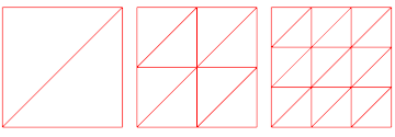
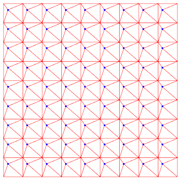
1. nPts, either a number n or pair of numbers { m, n }, specifies a grid or mesh of rectangular cells subdividing the plot domain. $$\begin{align} x_1 < x_2 < \cdots < x_m \\ y_1 < y_2 < \cdots < y_n \end{align}$$ Initially each rectangular cell is subdivided into two triangles by its diagonal from the lower left corner $(x_i,y_j)$ to the upper right $(x_{i+1},y_{j+1})$.

   • MaxRecursion -> 0: The initial triangles remain the basis of the triangulation if extrapoints are added.
   • MaxRecursion -> n, n > 0: The initial rectangles remain the basis of the triangulation if extrapoints are added.

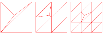
2. From extrapoints, a list { { x1, y1 }, ... } of points, each point is added in turn. When a point $P$ is placed inside a triangle, the triangle is subdivided into the three triangles formed by the point $P$ and each of the edges of the triangle, with two exceptions:

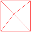
   • If MaxRecursion is at least 1, then when the first point added to a rectangular cell, the diagonal is removed and the cell is divided into four triangles formed by the point $P$ and each of the edges.
   • If the surface bends too much, then sometimes further subdivisions are made.

3. If MaxRecursion is set greater than 0, then begining with the triangles in unaltered mesh cells (those without any extrapoints), the triangles are usually subdivided by bisecting the edges and connecting the points of bisection at one edge. For mesh cells altered by having some extrapoints placed in it, recursived subdivision seems to "invade" one its triangles when one of the triangle's edges is bisected (which happens when it is adjacent to a triangle being subdivided). Such triangles are then subject to further recursive subdivision.

Notes:

• When a point is place in a triangle, the angles at existing vertices are divided, tending to make narrow triangles.
• In recursive subdivision, the subdivision happens on the edges of the triangles (except when invading a triangle formed from extrapoints), and the angles at the vertices tend not be divided.
  • The lines $x = x_i$ and $y = y_j$ are always present, although they will usually be divided into smaller segments by recursive subdivision. However, adding extrapoints never seems to cause them to be divided. If an added point lies on one of the lines, it seems to be ignored.
• Adding many extrapoints in a cell has a tendency to create small angles at the vertices, which render like "ice-crystals."

Below I give some evidence for these assertions.

The problem with narrow triangles

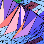
One problem with narrow triangles can be seen in the changes in angle of the surface. The orientation of many of the triangles below do not align with the normal vector of the surface. When VertexNormals is turned on, the rendering uses interpolation to figure out how to light the surface so that it appears smooth. The algorithm cannot accurately render the surface when the normals to the triangles vary so wildly.

Recursive subdivision in the presence of extra points

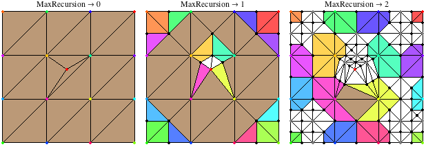
One extra point added. Below, first the top, and then the right and left edges of the middle cell are bisected, which enables subdivision of the center cell.

Module[{tmpplot, nPts, plotpoints = 4, extrapoints = {{-0.03, 0.12}}},
 Grid@{
  Table[
   Block[{f = Sin[10 #1] Cos[10 #2] &},
    Show[
     tmpplot[r] = project2D@testPlot[plotpoints, extrapoints, r],
     Graphics[
      {PointSize[Medium],
       Cases[tmpplot[r], GraphicsComplex[p_, g_] :>
        (nPts[r] = Length[p];
         Point[p, VertexColors ->
          vColors[plotpoints, Length[extrapoints], If[r > 0, nPts[r - 1], 0]]])]}
    ],
    AxesLabel -> {"x", "y"}, 
    PlotLabel -> Row[{"MaxRecursion \[Rule] ", r}], 
    ImageSize -> 200]],
   {r, 0, 2}]}
]

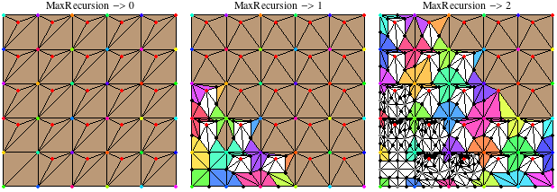
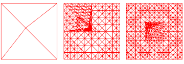
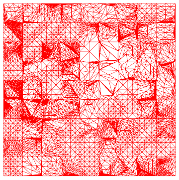
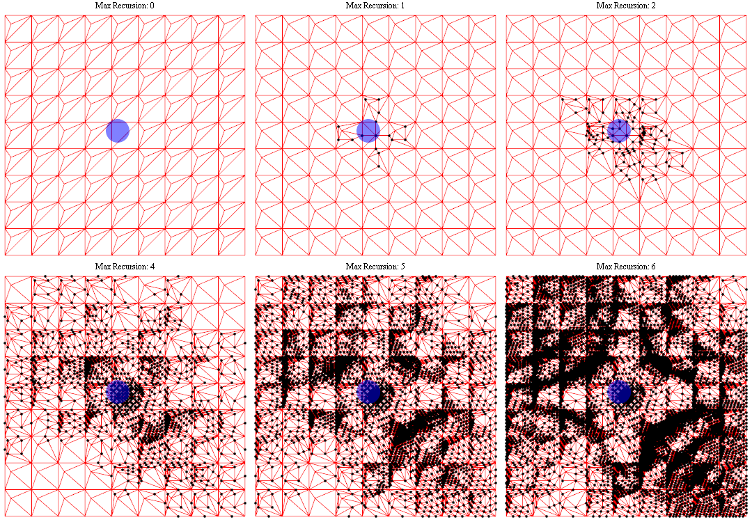
Many extra points. Adding points in adjacent cells slows (and alters) the recursive subdivision. The propagation depends on the function being plotted. (See also Simon Wood's beautiful animation.)

Module[{tmpplot, nPts, plotpoints = 6, extrapoints},
 extrapoints =
  Drop[
   Flatten[
    Table[{-0.03, 0.12} + 2 {i, j}/(plotpoints - 1), 
      {i, -2, 2}, {j, -2, 2}], 1], 1];
 Grid@
  {Table[
    Block[{f = Sin[10 #1] Cos[10 #2] &},
     Show[
      tmpplot[r] = project2D@testPlot[plotpoints, extrapoints, r],
      Graphics[
       {PointSize[Medium],
        Cases[tmpplot[r],
         GraphicsComplex[p_, g_] :>
          (nPts[r] = Length[p];
           Point[p, VertexColors ->
            vColors[plotpoints, Length[extrapoints], If[r > 0, nPts[r - 1], 0]]])]}
    ],
    AxesLabel -> {"x", "y"}, 
    PlotLabel -> Row[{"MaxRecursion -> ", r}], ImageSize -> 200, 
    PlotRange -> All]], {r, 0, 2}]}
]

Adding points to triangles

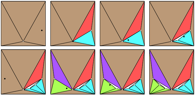
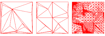
Below demonstrates what happens as each point in a list of extrapoints is processed. The black dot is the next point to be processed, and the triangle containing it is subdivided at the next step.

Block[{f = 1 &, x1, x2, y1, y2},
 {x1, x2} = 0.6 {-1, 1};
 {y1, y2} = 0.5 {-1, 1};(*reset domain for testPlot*)
 Module[
  {extrapoints = # + {0, -0.4} & /@ 
    Take[myExtrapoints[2, 0], 8]},
  Grid[Partition[#, 4]] &@
   Table[
    Show[
     project2D@testPlot[2, Take[extrapoints, n], 1],
     Graphics[
      {LightGray, Point[Take[extrapoints, n]],
       If[n < Length[extrapoints],
        {Black, PointSize[Medium], Point[extrapoints[[n + 1]]]}, {}]}
     ],
     ImageSize -> 150, AspectRatio -> 1],
    {n, Length[extrapoints]}]
 ]
]

The OP's Example

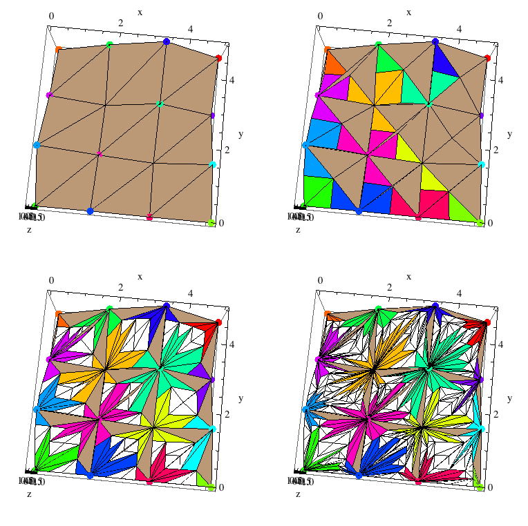
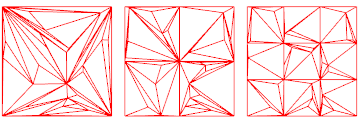
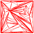
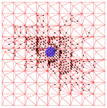
We can see that when the points generated by recursive subdivision are added to a plot as extrapoints, the triangles are not subdivided in the same way that was used to generate the points. Many points are placed in each rectangular cell. As a result, many narrow corners are created. Further, having points in each cell inhibits recursive subdivision.

The following shows the OP's function with PlotPoints set to 4 and extrapoints taken from those added by MaxRecursion set to 0, 1, 2, 3. The original 16 vertices are colored a hue. A triangle is colored the same color as one of the 16 vertex if contains exactly one of the vertices. If it contains two or more, it is colored brown. If it contains none of the 16 original vertices, the triangle is colored white.

f[x_, y_] := Cos[y]^3 Sin[x]^2 + Cos[x] Sin[y];
plotVP = {1.3, -2.4, 2}; plotVV = {0, 0, 1};
Module[{extrapoints, tmpplot},
 Table[
  extrapoints =
   Reap[
    Plot3D[f[x, y], {x, 0, 5}, {y, 0, 5},
     PlotPoints -> 4, MaxRecursion -> R, 
     EvaluationMonitor :> Sow[{x, y}]]][[-1, 1]];
  Show[
   tmpplot =
    Plot3D[f[x, y], {x, 0, 5}, {y, 0, 5},
     Mesh -> None, PlotPoints -> {4, extrapoints}, MaxRecursion -> 0,
     NormalsFunction -> None] /.
      Polygon[l_] :>
       ({If[Length[#] == 1, Hue[5 First[#]/16], 
          If[Length[#] == 0, White, Lighter@Brown]] &@
           Cases[#, Alternatives @@ Range[16]], 
         EdgeForm[Black], Polygon[#]} & /@ l),
   Graphics3D[
    Cases[tmpplot,
     GraphicsComplex[p_, g_] :>
      GraphicsComplex[p, {PointSize[Large], Point[Range[16],
       VertexColors -> (Hue[Mod[5 #/16, 1]] & /@ Range[16])]}]]
  ],
  AxesLabel -> {"x", "y", "z"}, SphericalRegion -> True, 
  ViewPoint -> Dynamic[plotVP],
  ViewVertical -> Dynamic[plotVV], Lighting -> {{"Ambient", White}}, 
  ImageSize -> 250], {R, 0, 3}]
]

An Example Application

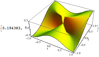
This is an edit of the previous work. Understanding better now how adding points works, I can show how in this case that adding extrapoints helps. The function is $f(x,y)={x^2y \over x^4+y^2}$. It has a ridge, almost a cliff, along $y = \pm x^2$ that becomes infinitessimally thin at the $z$-axis. If a subdivision results in a triangle spanning across the ridge, a gap appears. Also, the cliff is nearly vertical near the origin and the Front End can get confused about which side of a component polygon is up.

Here is the standard output of Plot3D:

Plot3D[(x^2 y)/(x^4 + y^2), {x, -1, 1}, {y, -1, 1}, 
  PlotStyle -> FaceForm[Yellow, Blue], Mesh -> None, 
  AxesLabel -> {"x", "y", "z"}, ImageSize -> 250] // AbsoluteTiming

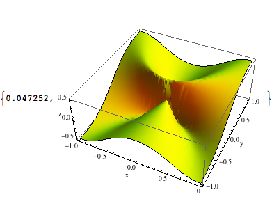
Even upping the PlotPoints and MaxRecursion does not eliminate the gap:

Plot3D[(x^2 y)/(x^4 + y^2), {x, -1, 1}, {y, -1, 1}, 
  PlotPoints -> {50, 51}, 
  PlotStyle -> FaceForm[Yellow, Blue], 
  Mesh -> None, MaxRecursion -> 3, 
  AxesLabel -> {"x", "y", "z"}, ImageSize -> 250] // AbsoluteTiming

If the subdivision could be along the parabola $y=x^2$ instead of the default, perhaps a more accurate graph might be generated. If points were placed somewhat as they were above in the section "Adding points to triangles", then an approximation to the parabola can be made by the segments connecting them. (See also myExtrapoints in the Utility functions below.) If in each rectangular cell, the outer two points were close to the edge of the rectangle, then the ridge would be nearly continously connected, except for a very small gap at the mesh lines $x = x_i$. A major problem is that the function $f$ is undefined at $(0,0)$, so something special has to be done near the origin. We put two points very close on either side of the origin. There are also some further points added to extrapoints to help keep a subdivision from crossing the ridge. The result is passible, and the computation is not much slower than the default Plot3D. The ridge is evident, but there are still shadows on the surface.

Module[{plotpoints = 15, extrapoints},
 extrapoints = myExtrapoints[plotpoints];
 Plot3D[(x^2 y)/(x^4 + y^2), {x, -1, 1}, {y, -1, 1}, 
  Mesh -> None, PlotStyle -> FaceForm[Yellow, Blue], 
  PlotPoints -> {{plotpoints + 1, plotpoints}, extrapoints}, 
  MaxRecursion -> 2, AxesLabel -> {"x", "y", "z"}, 
  SphericalRegion -> True, ImageSize -> 300]
 ] // AbsoluteTiming

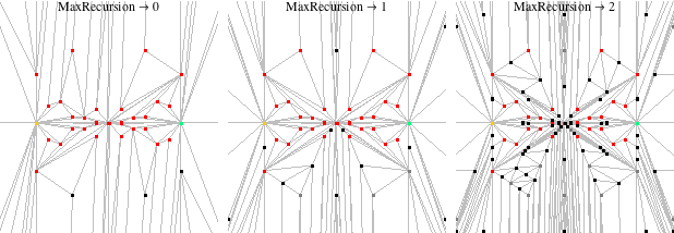
This shows the extrapoints and what happens under recursive division near the origin. (Note PlotRange->{{-0.1,0.1},{-0.01,0.01}}.)

Module[{tmpplot, plotpoints = 15, extrapoints, nPts, nExtra},
 extrapoints = myExtrapoints[plotpoints];
 nExtra = Length[extrapoints];
 Grid@
  {Table[
    Block[{f},
     f[x_, y_] := (x^2 y)/(x^4 + y^2);(*redefine for testPlot*)
     Show[
      tmpplot[r] =
       project2D@testPlot[{plotpoints + 1, plotpoints}, extrapoints, r] /.
        EdgeForm[_] -> EdgeForm[GrayLevel[0.75]],
      Graphics@
       Cases[tmpplot[r],
        GraphicsComplex[p_, g_] :>
         (nPts[r] = Length[p];
          Point[p, 
           VertexColors -> 
            vColors[plotpoints, nExtra, If[r > 0, nPts[r - 1], 0]]])],
      PlotLabel -> Row[{"MaxRecursion \[Rule] ", r}], ImageSize -> 200,
      PlotRange -> {{-0.1, 0.1}, {-0.01, 0.01}}, AspectRatio -> 1]],
    {r, 0, 2}]}
]

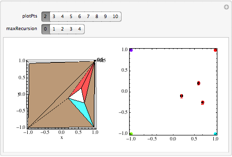
A Manipulate toy

I had a dynamic example originally, which I here replace with a Manipulate that also allows for controlling PlotPoints and MaxRecursion. I thought I might as well share it.

Manipulate[
 Grid[
  {{Dynamic@
     Show[
      tmpplot =
       testPlot[plotPts, LP = localPts, maxRecursion],
      Axes -> True, AxesLabel -> {"x", "y", "z"},
      SphericalRegion -> True, ViewPoint -> Dynamic[plotVP],
      ViewVertical -> Dynamic[plotVV],
      Lighting -> {{"Ambient", White}}, ImageSize -> 200],
    LocatorPane[
     Dynamic[localPts],
     Dynamic@
      Show[
       actualPts2D[tmpplot, plotPts], ImageSize -> 200, Frame -> True],
     LocatorAutoCreate -> True,
     Appearance -> (Style[#, Red] & /@ Range[Length[localPts]])]}}
  ],
 {{localPts, {{0.2, -0.1}, {0.7, -0.25}, {0.6, 0.2}}}, None},
 {tmpplot, None},
 {plotPts, Range[2, 10], SetterBar},
 {maxRecursion, Range[0, 4]}, SaveDefinitions -> True]

Utility Functions

Plotting functions. testPlot generates a 3D plot. Others (actualPts2D and project2D) map parts of the output to 2D.

f[x_, y_] := Cos[10 y] Sin[10 x];(*default function*)
plotVP = {0, 0, 10};
plotVV = {0, 1, 0};(*ViewPoint,ViewVertical*)
colorFn[i_, n_] := 
 Hue[Mod[(If[CoprimeQ[n, #], #, # + 1] &@Floor[n/3.5]) i/n, 1]];
vColors[plotpoints_, nExtra_, nOld_] :=(*vertex coloring*)
 (colorFn[#, plotpoints^2] & /@ 
   Range[plotpoints^2])~Join~ConstantArray[Red, nExtra]~Join~
   If[nOld >= 1, 
    ConstantArray[Gray, nOld - plotpoints^2 - nExtra], {}];

{x1, x2} = {-1, 1};
{y1, y2} = {-1, 1};(*default domain for testPlot*)
testPlot[plotPts_, localPts_, maxRecursion_, opts___] :=
 Plot3D[f[x, y], {x, x1, x2}, {y, y1, y2},
  Mesh -> None, PlotPoints -> {plotPts, localPts},
  MaxRecursion -> maxRecursion, NormalsFunction -> None,
  PlotRange -> All, Axes -> False, opts] /. Polygon[l_] :>
({If[Length[#] == 1,
     FaceForm[Lighter@colorFn[#, plotPts^2], Darker@Lighter@colorFn[#, plotPts^2]], 
    If[Length[#] == 0, 
     FaceForm[White, Black], 
     FaceForm[Lighter@Brown, Darker@Brown]]] &@
      Cases[#, Alternatives @@ Range[plotPts^2]], 
  EdgeForm[Black], Polygon[#]} & /@ l);

actualPts2D[plot_, plotPts_] :=
(*get the points from a Plot3D and converts them to 2D coords*)
 Graphics[
  Cases[plot,
   GraphicsComplex[p_, g_] :>
    GraphicsComplex[Most /@ p,
     {PointSize[0.07/plotPts],
      Point[Range[Length[p]], 
       VertexColors -> (colorFn[#, plotPts^2] & /@ Range[plotPts^2])]}]
  ]
 ];

project2D[plot_] :=(*project a Plot3D output onto xy plane*)
 Show[
  plot /.
  {GraphicsComplex[p_, g_] :> GraphicsComplex[Most /@ p, g]} /.
   Graphics3D[g_, opts___] :> 
    Graphics[g, FilterRules[opts, Options[Graphics]]],
  PlotRange -> Automatic
 ]

The extra points for the example surface. Somewhat through trial and error, so programmatically a bunch of special cases. myExtrapoints[plotpoints] generates extra points for each cell along the ridge, for roughly $-0.2 < x < 0.2$; $x = 0$ is a special case. It needs plotpoints to be even and the domain to be symmetric about $x=0$.

myExtrapoints[plotpoints_, 0 | 0.] :=(*center at origin*)
 Join @@
  {{#, #^2} & /@
   ({-1/100 , 999/1000 , 1/100 , 1/3 , 2/3 , -999/1000 , -1/3 , -2/3 }/plotpoints),
   {#, 10 #^2} & /@ Table[i/plotpoints/6, {i, -1, 1, 2}],
   {#, #^2/2} & /@ Table[i/plotpoints/6, {i, -5, 5, 2}],
   {{1/2, 1/10}, {-1/2, 1/10}, {0, 1/5}}/plotpoints
  }

myExtrapoints[plotpoints_, ctr_] :=(*generic center*)
 Join @@
  {Table[{x, x^2},
   {x, If[ctr > 0, Reverse@#, #] &@
    {ctr - 1/plotpoints + 1/plotpoints/1000, 
     ctr, ctr + 1/plotpoints - 1/plotpoints/1000}}], 
   {#, #^2 +  1/plotpoints/4} & /@ 
    {ctr - 1/plotpoints/2, ctr + 1/plotpoints/2},
   {{ctr, ctr^2 + 2/plotpoints/3}}
  }

myExtrapoints[plotpoints_?OddQ] :=
 #~Join~({1, -1} # & /@ #) &@
  Flatten[
   Table[
    myExtrapoints[plotpoints, c],
    {c, Round[-0.2, 2/plotpoints], -(Round[-0.2, 2/plotpoints]),2/plotpoints}], 1]