39
$\begingroup$

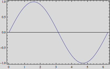
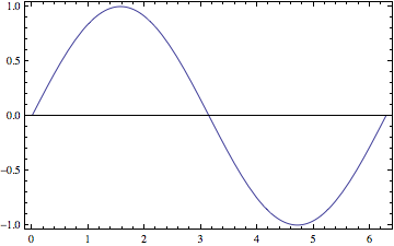
I frequently generate framed plots like this:

Plot[Sin[x], {x, 0, 2 π}, Frame -> True]

enter image description here

Is there an easy way to change the background color of the framed region only?

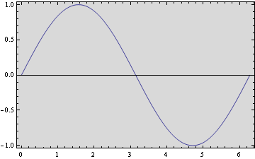
Specifying the Background option unfortunately changes the background color of the entire plot, not just the framed region:

Plot[Sin[x], {x, 0, 2 π}, Frame -> True, Background -> LightGray]

enter image description here

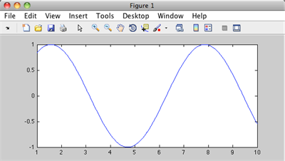
Also, is there a way to make figures look like MATLAB's default figure style, i.e. a white background surrounded by a gray frame (see below)?

MATLAB figure

$\endgroup$
8
  • 3
    $\begingroup$ See related: stackoverflow.com/questions/6303500/… $\endgroup$
    – Eli Lansey
    Commented Feb 24, 2012 at 14:36
  • $\begingroup$ The answers from stackoverflow.com/questions/6303500/… have been move here as a result of merging. $\endgroup$
    – Mr.Wizard
    Commented Feb 24, 2012 at 17:31
  • $\begingroup$ wow... it has been a while since I've been to stack overflow. But now I come back and my question has been migrated here and given credit to someone else... @Mr.Wizard, what's going on here? How do I find my original post? $\endgroup$
    – jmlopez
    Commented Mar 29, 2012 at 19:03
  • $\begingroup$ @jmlopez I am new to moderating but I am trying to do the best job I can. When a duplicate question was posted here (this one) I wanted to combine the two rather than cover old ground. Even at the time I was uncertain how to handle it; normally I would close the new question as a duplicate of the old, but it was suggested to me to keep the new one instead, and since you appeared to have left StackExchange I did not argue. Please read the chat transcript to see how this played out. $\endgroup$
    – Mr.Wizard
    Commented Mar 30, 2012 at 1:23
  • 2
    $\begingroup$ @Mr.Wizard it appears it was deleted, yet he retains the rep from it. $\endgroup$
    – rcollyer
    Commented Apr 8, 2012 at 2:39

7 Answers 7

37
$\begingroup$

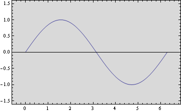
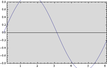
You can use the Prolog option with Scaled coordinates:

Plot[Sin[x], {x, 0, 2 π}, Frame -> True,
 Prolog -> {LightGray, Rectangle[Scaled[{0, 0}], Scaled[{1, 1}]]}
]

Mathematica graphics

Note: Using scaled coordinates lets this work for any PlotRangePadding, and with PlotRangePadding->False:

Plot[Sin[x], {x, 0, 2 π}, Frame -> True, 
 Prolog -> {LightGray, Rectangle[Scaled[{0, 0}], Scaled[{1, 1}]]}, 
 PlotRangePadding -> .6]

Mathematica graphics

Plot[Sin[x], {x, 0, 2 π}, Frame -> True, 
 Prolog -> {LightGray, Rectangle[Scaled[{0, 0}], Scaled[{1, 1}]]}, 
 PlotRangePadding -> -.2, PlotRangeClipping -> False]

Mathematica graphics

$\endgroup$
1
  • $\begingroup$ Very helpful. Thank you both! $\endgroup$
    – Cassini
    Commented Feb 24, 2012 at 14:37
27
$\begingroup$

After playing around for a while with various graphics and frame options...
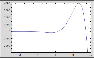
I decided to take the simplest option - your polygon one:

Framed[Plot[Sin[x] Exp[x], {x, 1, 10}, Frame -> True, 
  PlotRangePadding -> None, Axes -> False, 
  Prolog -> {White, Rectangle[Scaled[{0, 0}], Scaled[{1, 1}]]}], 
 Background -> LightGray]

An example image generated from the above code

$\endgroup$
3
  • 7
    $\begingroup$ This works because Plot sets PlotRangeClipping -> True by default. (A good choice -- it keeps curves from drawing beyond the frame.) Using Scaled instead of ImageScaled would be better, since the Scaled coordinate system naturally corresponds to plot range (ie, the region inside the frame.) $\endgroup$ Commented Jun 10, 2011 at 14:13
  • $\begingroup$ @Brett: Thanks Brett. Using Scaled is by far the better choice. Too many graphics/image options and I always forget which is which. $\endgroup$
    – Simon
    Commented Jun 10, 2011 at 23:56
  • $\begingroup$ @Brett and @Simon: I edited my post in order to add a solution based on your ideas. This gives me more control over my custom labels and graphics. Thank you for your answers. $\endgroup$
    – jmlopez
    Commented Jun 11, 2011 at 20:57
14
$\begingroup$

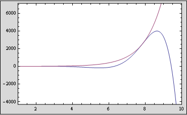
You could also do:

Framed[Plot[{Sin[x] Exp[x], Exp[x]}, {x, 1, 10}, 
       Frame -> True, 
       Axes  -> False, 
       PlotRangePadding -> None, 
       Filling          -> {1 -> Top, 1 -> Bottom}, 
       FillingStyle     -> White], 
       Background       -> LightGray]

enter image description here

Edit

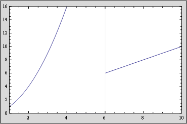
I suspected problems when the function is not defined in the full range, but found it is not the case:

Framed[Plot[{Piecewise[{{x^2, x < 4}, {x, x > 6}}]}, {x, 1, 10}, 
       Frame -> True, 
       Axes  -> False, 
       PlotRangePadding -> None, 
       Filling          -> {1 -> Top, 1 -> Bottom}, 
       FillingStyle     -> White], 
       Background       -> LightGray]  

enter image description here

$\endgroup$
3
  • $\begingroup$ +1 The hack even works if you want to fill down in color and have the rest white. Framed[Plot[{Piecewise[{{x^2, x < 4}, {x, x > 6}}]}, {x, 1, 10}, Frame -> True, Axes -> False, PlotRangePadding -> None, Filling -> {1 -> Top, 1 -> Bottom}, FillingStyle -> {White, Blue}, ImageSize -> Large], Background -> LightGray] $\endgroup$
    – Simon
    Commented Jun 10, 2011 at 13:35
  • $\begingroup$ @Simon Not so well. Try -x^2 instead of x^2 $\endgroup$ Commented Jun 10, 2011 at 13:43
  • $\begingroup$ The problem there is a combination of the PlotRange and the default default (0) for Piecewise... $\endgroup$
    – Simon
    Commented Jun 10, 2011 at 13:57
8
$\begingroup$

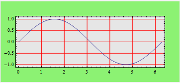
While Eli's answer is elegantly simple, it has a drawback: the Prolog objects are layered on top of GridLines, thus a background rectangle covers all the gridlines. So to come over this issue, here is my version of a background-and-frame.

The general background (gray) is defined by the outermost Frame's Background option (this way we won't cover GridLines), while the outer green frame is defined as a FilledCurve (using ImageScaled and Scaled coordinates), put in an independent Graphics object, and displayed with the final plot via Show. There is at least one caveat: any options defined for a Plot object must be then forwarded to the Show, otherwise they mess up the result.

Framed[
 Show[
  Graphics[{
    Hue[.3, 1, 1, .5], 
    FilledCurve[{
        {Line[ImageScaled /@ {{0, 0}, {1, 0}, {1, 1}, {0, 1}}]},
        {Line[Scaled /@ ({{0, 0}, {1, 0}, {1, 1}, {0, 1}})]}
       }],
    }],
  Plot[Sin[x], {x, 0, 2 \[Pi]}], (* this is the main plot, options given to Show *)
  ImagePadding -> 30, Frame -> True, GridLines -> Automatic, 
  GridLinesStyle -> Red
  ],
 Background -> [email protected], FrameMargins -> 0, FrameStyle -> None]

Mathematica graphics

You might wonder why I didn't put the FilledCurve into the Plot's Prolog: well, Prolog cannot handle coordinates that are out of the defined PlotRange, thus ImageScaled coordinates out of the plot's frame won't show at all.

$\endgroup$
1
  • $\begingroup$ This is also a very ellegant solution for those annoying cases where PlotRangeClipping will fail to fully clip the corners of lines when they meet the frame. $\endgroup$ Commented Apr 24, 2017 at 18:17
7
$\begingroup$

This is how I would do it:

passepartout[plot_, opt : OptionsPattern[]] := With[{
   p = Show[plot, PlotRangePadding -> None]
   },
  Show[Show[
    Graphics[{((Background /. Options[plot]) /. 
        Background -> Transparent), 
      Apply[Rectangle, Transpose[PlotRange /. Quiet@AbsoluteOptions[p]]]}], 
    p, Options[p]],
   opt]
  ]

This function should be able to take any Graphics object as its argument "plot". It uses whatever Background plot has been given beforehand, and then adds the frame according to the options Background and ImagePadding supplied to the passepartout function.

For example, start with a plot

p = Plot[Sin[x], {x, 1, 10}, Frame -> True, Axes -> False, Background -> Yellow]

(I added a yellow background, but that's just for illustration and is completely optional). To get what you're looking for, just say

passepartout[p, ImagePadding -> 30, Background -> LightGray]
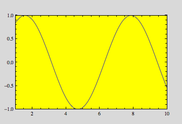
Output of the previous command

To make the frame thicker or asymmetric, use the standard ImagePadding syntax. You can also add other options such as AspectRatio to passpartout.

In the passepartout function, I use AbsoluteOptions to extract the PlotRange that determines the "passepartout opening." You could replace this by Options to speed things up, but the advantage of using AbsoluteOptions is that it also works for arbitrary Graphics, such as

p = Graphics[Circle[], Background -> Yellow]
$\endgroup$
5
$\begingroup$

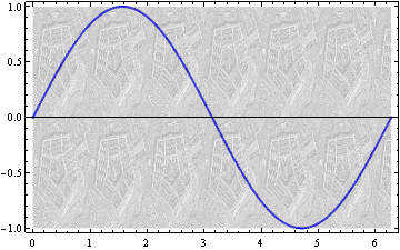
I'll add another way of combinig a plot with an image :

gr = Graphics[{
       Opacity[0.4], Texture[ExampleData[{"AerialImage", "Pentagon"}]], 
       Polygon[{{0, -1}, {2 Pi, -1}, {2 Pi, 1}, {0, 1}}, 
       VertexTextureCoordinates -> {{0, -1}, {2 Pi, -1}, {2 Pi, 1}, {0, 1}}]}]
Show[Plot[ Sin[x], {x, 0, 2 Pi}, PlotStyle -> {Blue, Thick}, Frame -> True], gr] 

enter image description here

$\endgroup$
3
  • 1
    $\begingroup$ You needed to rescale the sine curve to fit the image dimensions. This is not practical. Why don't you put the image into a Raster and position the Raster to fill up the whole plot range (Scaled)? Or why don't you tile a Texture onto a background Rectangle? $\endgroup$
    – Szabolcs
    Commented Feb 24, 2012 at 18:20
  • $\begingroup$ @Szabolcs Good point! Not sure if Raster would yield a better solution, since there might be still some arrangements to do. But hope this completely different approach is worthy of note. $\endgroup$
    – Artes
    Commented Feb 24, 2012 at 19:30
  • 2
    $\begingroup$ Plot[Sin[x], {x, 0, 2 Pi}, Prolog -> {{Raster[ ExampleData[{"AerialImage", "Pentagon"}, "Data"]/ 255., {Scaled[{0, 0}], Scaled[{1, 1}]}]}}, Frame -> True] $\endgroup$
    – Szabolcs
    Commented Feb 24, 2012 at 19:37
5
$\begingroup$

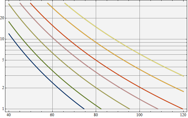
It is possible to combine a background PlotRange fill using the Scaled Rectangle approach with GridLines by specifying the undocumented option Method -> {"GridLinesInFront" -> True}. If it is desirable to place the plot lines over the grid lines we can move or copy the Line primitives into an Epilog option.

Mathematica graphics

gr = LogPlot[
  {5 (80/x)^4, 5 (55/x)^4, 12 (40/x)^4, 15 (80/x)^4, 9 (80/x)^4, 15 (55/x)^4, 9 (55/x)^4},
  {x, 40, 120},
  PlotStyle -> Map[Directive[Thick, ColorData[14]@#] &, {2, 6, 7, 4, 3, 1, 5}],
  GridLines -> Automatic,
  PlotRange -> {1, 33},
  Frame -> True,
  PlotRangePadding -> {Automatic, 0.1},
  Prolog -> {GrayLevel[0.95], Rectangle[Scaled[{0, 0}], Scaled[{1, 1}]]},
  Method -> {"GridLinesInFront" -> True},
  ImageSize -> 500
];

Show[gr,
  Epilog -> (gr[[1, 1]] /.
    {style__, x_Line} :> {{Black, Opacity[0.5], AbsoluteThickness[3], x}, style, x})]
$\endgroup$
4
  • $\begingroup$ This is promising. Is there also a way to get the plot legend back on top? $\endgroup$
    – Thijs
    Commented Jul 22, 2015 at 10:16
  • 1
    $\begingroup$ @Thijs (1) which version of Mathematica are you using? (2) Legends are normally placed to the side and should not be an issue; can you give me a code example where you have a problem? $\endgroup$
    – Mr.Wizard
    Commented Jul 22, 2015 at 10:25
  • $\begingroup$ I use Mathematica 10. You are right. I put the legend inside the plot. How can I share a simplified code example with you? It is too long for a comment. $\endgroup$
    – Thijs
    Commented Jul 22, 2015 at 10:33
  • $\begingroup$ @Thijs I am in Chat. $\endgroup$
    – Mr.Wizard
    Commented Jul 22, 2015 at 10:37

Your Answer

By clicking “Post Your Answer”, you agree to our terms of service and acknowledge you have read our privacy policy.

Not the answer you're looking for? Browse other questions tagged or ask your own question.