18
$\begingroup$

I have a list of $\{x,y,z\}$ pairs representing points in $R^3$. For every unique value of $z$ there are many $\{x,y\}$ pairs defining a polygon/contour in that particular $z$-plane. My dataset looks like this:

Take[ptv, 3]
(*{{61.52, -217.26, -80}, {63.48, -217.64, -80}, {65.43, -217.64, -80}}*)

These are coordinates of points residing on the $z=-80$ plane. There are other pairs for $z=-75$, $z=-70$, etc. Therefore ptv is of the form:

ptv: {{$x_1,y_1,-80$}, {$x_2,y_2,-80$}, ..., {$x_k,y_k,-80$}, ..., {$x_1,y_1,-75$}, ..., {$x_m,y_m,-75$}, ...}

My goal is to create a 3D surface where:

(1). the points in every $z$-plane are connected into a polygon/contour and (2). the points in every $z$-plane are connected with their neighbors in the immediately above and below plane.

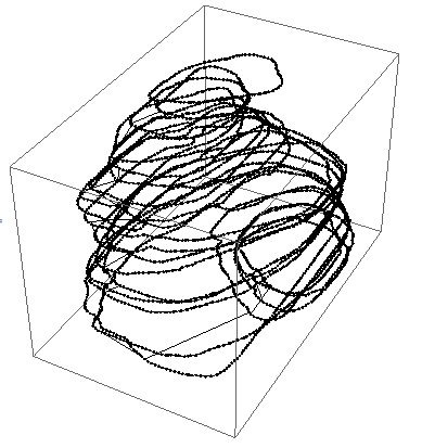
I have achieved (1), via:

Graphics3D[{Line[ptv], Point /@ ptv}]

The result looks like this: Plot1
If I, instead, use:

ListSurfacePlot3D[ptv, AxesLabel -> {"x","y","z"}]

Then I get some ugly artifacts (edges at the boundaries of the volume) as shown here: Plot2
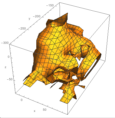
Whereas, I was expecting a more "smooth" surface without any "openings". Any hints on:

  1. Whether ListSurfacePlot3D[] is the proper function to use (i.e. in the documentation it is mentioned that ListSurfacePlot3D[] may "fold" over; perhaps this is why I'm experiencing these ruffles?) or
  2. What other alternatives are there to consider ?

EDIT 1: Minimally working example:

ClearAll["Global`*"];
ptv = Import["http://leaf.dragonflybsd.org/~beket/ptvgeom/ag1", "Table"]
ListSurfacePlot3D[ptv, AxesLabel -> {"x", "y", "z"}]

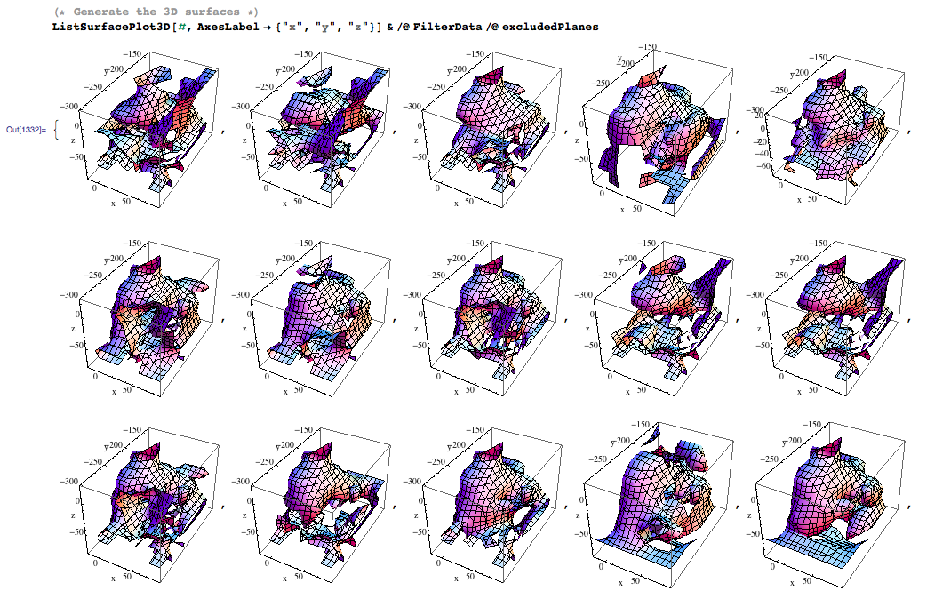
EDIT 2: I excluded random $z$-planes to explore the dependence of the produced surfaces on my dataset. There is considerable visual variability in the output, including some very irregular images. Here is the code:

(* Identify the values of z-planes *)
planes = ({x, y, z} = #; z)& /@ ptv // Union;

(* Generate some random sequences with z-planes-to-be-excluded *)
excludedPlanes = Table[
    RandomSample[planes, RandomInteger@{1, 4}],
    {k, 1, 20}]] // Union // Reverse;

(* Filter data by discarding points residing on excluded planes *)
FilterData[p_] := Select[ptv,
    Function[v, And@@(Unequal[v, #]& /@ p)][Last[#]]&]

(* Generate the 3D surfaces *)
ListSurfacePlot3D[#, AxesLabel->{"x","y","z"}]& /@ FilterData/@ excludedPlanes

And here is a screenshot:
enter image description here


Problem

Although Dr.belisarius has given a solution, however, which lost the geometry continuty.
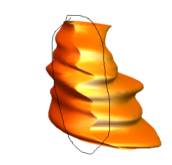
enter image description here

In addition, the contour didn't pass the interpolating points.

f = BSplineFunction[Most /@ t[[1]]]
Show[{ListPlot[Most /@ gb[[1]], PlotTheme -> "Classic"], 
      ParametricPlot[f[t], {t, 0, 1}, PlotTheme -> "Classic"]}]
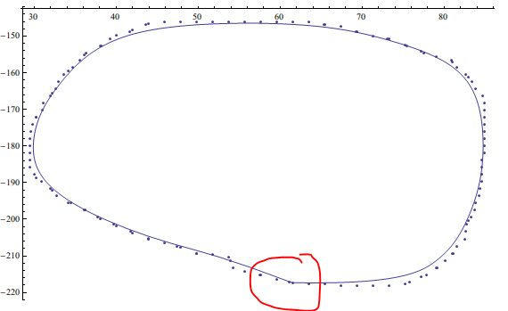
enter image description here

$\endgroup$
8
  • $\begingroup$ Since this is my first post here, I will allow myself a question: what did I do wrong and got down-voted ? If I hover my mouse in the 'downvote' image I get a tooltip saying that the question lacks research effort, is unclear or not useful. So which one of three is it ? $\endgroup$
    – stathisk
    Commented Aug 17, 2013 at 19:55
  • 2
    $\begingroup$ Sorry, I didn't understand I had to upload my dataset. Is this what 'MWE' mean? I assumed all I needed was to include the 2nd code-snippet with ListSurfacePlot3D[]. Thanks belisarius! $\endgroup$
    – stathisk
    Commented Aug 17, 2013 at 20:35
  • 1
    $\begingroup$ You're welcome. MWE means "a minimal working example". Upload the minimal dataset you can generate that shows your problem. $\endgroup$ Commented Aug 17, 2013 at 20:36
  • 1
    $\begingroup$ If you are asking about not very smooth edges, Well, the help says attempts to reconstruct smooth surfaces defined by sets of points notice the word attempts :) I tried to find what Method it uses for interpolation, but could not find, other than Automatic. I tried few and none of them were accepted. If someone can find the Method that can be used there, that will be something to try. But like for many Mathematica functions, the Method option used seems to be a mystery item to find easily. $\endgroup$
    – Nasser
    Commented Aug 17, 2013 at 23:11
  • 4
    $\begingroup$ @belisarius your graph is spectacular! Thanks! I will study your methodology as it is very new to me. PS. For completeness / archiving reasons, I mention that this volume is a radiotherapy planning treatment volume of a lung tumor. $\endgroup$
    – stathisk
    Commented Aug 18, 2013 at 1:35

2 Answers 2

16
$\begingroup$

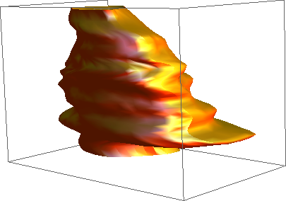
The natural way to go is BSplineFunction[]. The problem is that it needs a rectangular array of data as input and you collected a different number of points for each z plane.

So what we will do is to get an interpolating function for each z == const plane and generate an equal number of points at each plane. To be somewhat more clever, we could generate evenly spaced points along each curve, but that small modification is left as an exercise.

Please note that the Spline Degree determines if the curve pass along your points exactly, or is just a smoothed approximation.

ClearAll["Global`*"];
ptv = Import["http://leaf.dragonflybsd.org/~beket/ptvgeom/ag1", "Table"];
Needs["DifferentialEquations`InterpolatingFunctionAnatomy`"]; 

gb = GatherBy[ptv, Last];
f[k_InterpolatingFunction, p_] := 
   k[p (Length @@ InterpolatingFunctionCoordinates[k] - 1) + 1]
t = Append[#, First@#] & /@ 
     Transpose@ Table[{f[Interpolation[#[[All, 1]]], p], 
                       f[Interpolation[#[[All, 2]]], p], #[[1, 3]]}& /@ gb,
                      {p, 0, 1, 0.005}];
s = BSplineFunction[t];
ParametricPlot3D[s[u, v], {u, 0, 1}, {v, 0, 1}, 
                 PlotStyle -> {Orange, Specularity[White, 10]}, 
                 Axes -> None, Mesh -> None]

Mathematica graphics

$\endgroup$
9
  • $\begingroup$ For some reason I forgot about BSplineFunction[] and spent a good time trying to reinvent it :) $\endgroup$ Commented Aug 18, 2013 at 4:18
  • $\begingroup$ This is not fair. You are supposed to do this without using "DifferentialEquationsInterpolatingFunctionAnatomy" !! $\endgroup$
    – Nasser
    Commented Aug 18, 2013 at 4:39
  • $\begingroup$ @Nasser No big deal, I'm using it only for counting the number of points at each z=constant plane. I already have them in gb, but using InterpolatingFunctionAnatomy seems more appropriate here $\endgroup$ Commented Aug 18, 2013 at 4:52
  • $\begingroup$ I was just kidding. I do not even know how you even did this, way over my head. $\endgroup$
    – Nasser
    Commented Aug 18, 2013 at 5:15
  • $\begingroup$ @Nasser Take a look at the initial comments. Perhaps they are clear enough to understand the code $\endgroup$ Commented Aug 18, 2013 at 15:52
6
+50
$\begingroup$

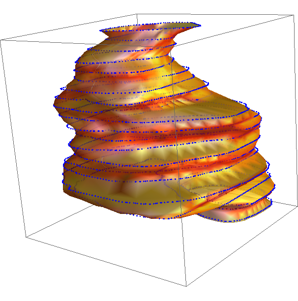
The following is a laborious procedure to build an homogeneous grid with angular symmetry. Not for the faint of heart, but it matches the original points quite well:

ptv = Import["http://leaf.dragonflybsd.org/~beket/ptvgeom/ag1",  "Table"];
Needs["DifferentialEquations`InterpolatingFunctionAnatomy`"];
gb = GatherBy[ptv, Last];
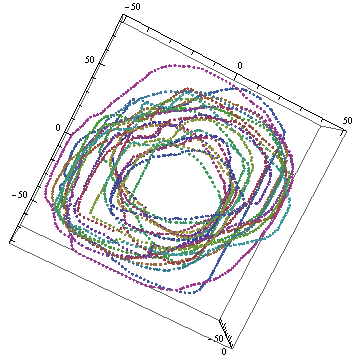
means = {1, 1, 0} # & /@ Mean /@ gb;
(*with the means subtracted the rings are almost concentric circles *)

ListPointPlot3D@(mi = MapIndexed[#1 - means[[#2[[1]]]] &, gb, {2}])

Mathematica graphics

(* Order them by angle *)
miOrd = SortBy[#, ArcTan[#[[1]], #[[2]]] &] & /@ mi;
(* find a nice curved path for them *)
miM = #[[First@FindCurvePath[#[[All, 1 ;; 2]]]]] & /@ mi;
(* get all of them winding in the same direction *)
miMdir = If[Tr@Sign@(Subtract @@@ Partition[ArcTan[#[[1]], #[[2]]] & /@ #, 2, 1]) > 0, #, 
          Reverse@#] & /@ miM;
(* and strting at the same angle *)
miMR = RotateLeft[#, First@Ordering[#, 1, 
       ArcTan[#1[[1]], #1[[2]]] < ArcTan[#2[[1]], #2[[2]]] &]] & /@ miMdir;
(* close the curves *)
miMRP = Append[#, #[[1]]] & /@ miMR;
(* calculate the interpolations *)
interp = Map[Interpolation[#] &, Transpose /@ miMRP, {2}];

(* Now we will calculate a homogeneous grid*)
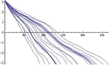
mm = Max[Length /@ Flatten[(InterpolatingFunctionCoordinates@#[[1]] & /@ interp), 1]];
Show @@ (Plot[
     ArcTan[#[[1]], #[[2]]] &@Through[#[x]], {x, 
      1, (Length @@ InterpolatingFunctionCoordinates@#[[1]] - 1)}, 
     PlotRange -> {{0, mm}, {-Pi, Pi}}] & /@ interp)

Mathematica graphics

findAngle[angle_, fun_] := 
 x /. FindRoot[ angle == ArcTan[#[[1]], #[[2]]] &@Through[#[x]], {x, 1, 1, 
      Length @@ InterpolatingFunctionCoordinates@#[[1]] - 1}] &@fun
radii = Quiet@ Outer[{#1, #2, Norm[#[[1 ;; 2]]] &@
       Through[(interp[[#2]])@findAngle[#1, interp[[#2]]]]} &, 
       Range[Pi - .001, -Pi + .001, -Pi/100], Range@Length@interp, 1];

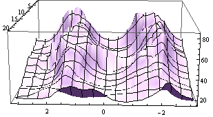
(* so, this is the grid *)
ListPlot3D[Flatten[radii, 1]]

Mathematica graphics

(* the cylindrical interpolation*)
g = Interpolation[Flatten[radii, 1]];

(*a scale conversion*)
conv[pt_] := {pt[[1]], pt[[2]], Rescale[pt[[3]], {-81, 25}, {1, Length@interp}]}

Show[Quiet@
  ParametricPlot3D[{# Cos@u, # Sin@u, v} &@g[u, v] + 
    Join[Through[(Interpolation /@ Transpose@means[[All, 1 ;; 2]])[
       v]], {0}], {u, -Pi, Pi}, {v, 1, 22}, BoxRatios -> 1, 
   PlotStyle -> {Opacity[.8], Orange, Specularity[White, 10]}, 
   Axes -> None, Mesh -> None],
 ListPointPlot3D[conv /@ ptv, PlotStyle -> {Blue, PointSize[Medium]}]]

Mathematica graphics

$\endgroup$

Your Answer

By clicking “Post Your Answer”, you agree to our terms of service and acknowledge you have read our privacy policy.

Not the answer you're looking for? Browse other questions tagged or ask your own question.