replaced http://mathematica.stackexchange.com/ with https://mathematica.stackexchange.com/
Source Link

The natural way to go is BSplineFunction[]. The problem is that it needs a rectangular array of data as input and you collected a different number of points for each z plane.

So what we will do is to get an interpolating function for each z == const plane and generate an equal number of points at each plane. To be somewhat more clever, we could generate evenly spaced points along each curveevenly spaced points along each curve, but that small modification is left as an exercise.

Please note that the Spline Degree determines if the curve pass along your points exactly, or is just a smoothed approximation.

ClearAll["Global`*"];
ptv = Import["http://leaf.dragonflybsd.org/~beket/ptvgeom/ag1", "Table"];
Needs["DifferentialEquations`InterpolatingFunctionAnatomy`"]; 

gb = GatherBy[ptv, Last];
f[k_InterpolatingFunction, p_] := 
   k[p (Length @@ InterpolatingFunctionCoordinates[k] - 1) + 1]
t = Append[#, First@#] & /@ 
     Transpose@ Table[{f[Interpolation[#[[All, 1]]], p], 
                       f[Interpolation[#[[All, 2]]], p], #[[1, 3]]}& /@ gb,
                      {p, 0, 1, 0.005}];
s = BSplineFunction[t];
ParametricPlot3D[s[u, v], {u, 0, 1}, {v, 0, 1}, 
                 PlotStyle -> {Orange, Specularity[White, 10]}, 
                 Axes -> None, Mesh -> None]
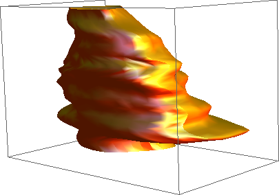
Mathematica graphics

The natural way to go is BSplineFunction[]. The problem is that it needs a rectangular array of data as input and you collected a different number of points for each z plane.

So what we will do is to get an interpolating function for each z == const plane and generate an equal number of points at each plane. To be somewhat more clever, we could generate evenly spaced points along each curve, but that small modification is left as an exercise.

Please note that the Spline Degree determines if the curve pass along your points exactly, or is just a smoothed approximation.

ClearAll["Global`*"];
ptv = Import["http://leaf.dragonflybsd.org/~beket/ptvgeom/ag1", "Table"];
Needs["DifferentialEquations`InterpolatingFunctionAnatomy`"]; 

gb = GatherBy[ptv, Last];
f[k_InterpolatingFunction, p_] := 
   k[p (Length @@ InterpolatingFunctionCoordinates[k] - 1) + 1]
t = Append[#, First@#] & /@ 
     Transpose@ Table[{f[Interpolation[#[[All, 1]]], p], 
                       f[Interpolation[#[[All, 2]]], p], #[[1, 3]]}& /@ gb,
                      {p, 0, 1, 0.005}];
s = BSplineFunction[t];
ParametricPlot3D[s[u, v], {u, 0, 1}, {v, 0, 1}, 
                 PlotStyle -> {Orange, Specularity[White, 10]}, 
                 Axes -> None, Mesh -> None]

Mathematica graphics

The natural way to go is BSplineFunction[]. The problem is that it needs a rectangular array of data as input and you collected a different number of points for each z plane.

So what we will do is to get an interpolating function for each z == const plane and generate an equal number of points at each plane. To be somewhat more clever, we could generate evenly spaced points along each curve, but that small modification is left as an exercise.

Please note that the Spline Degree determines if the curve pass along your points exactly, or is just a smoothed approximation.

ClearAll["Global`*"];
ptv = Import["http://leaf.dragonflybsd.org/~beket/ptvgeom/ag1", "Table"];
Needs["DifferentialEquations`InterpolatingFunctionAnatomy`"]; 

gb = GatherBy[ptv, Last];
f[k_InterpolatingFunction, p_] := 
   k[p (Length @@ InterpolatingFunctionCoordinates[k] - 1) + 1]
t = Append[#, First@#] & /@ 
     Transpose@ Table[{f[Interpolation[#[[All, 1]]], p], 
                       f[Interpolation[#[[All, 2]]], p], #[[1, 3]]}& /@ gb,
                      {p, 0, 1, 0.005}];
s = BSplineFunction[t];
ParametricPlot3D[s[u, v], {u, 0, 1}, {v, 0, 1}, 
                 PlotStyle -> {Orange, Specularity[White, 10]}, 
                 Axes -> None, Mesh -> None]
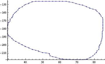
Mathematica graphics

added 56 characters in body
Source Link
Mr.Wizard
  • 273.1k
  • 34
  • 595
  • 1.4k

The natural way to go is BSplineFunction[]. The problem is that it needs a rectangular array of data as input and you collected a different number of points for each z plane.

So what we will do is to get an interpolating function for each z == const plane and generate an equal number of points at each plane. To be somewhat more clever, we could generate [evenly spaced points along each curve][1]evenly spaced points along each curve, but that small modification is left as an exercise.

Please note that the Spline Degree determines if the curve pass along your points exactly, or is just a smoothed approximation.

ClearAll["Global`*"];
ptv = Import["http://leaf.dragonflybsd.org/~beket/ptvgeom/ag1", "Table"];
Needs["DifferentialEquations`InterpolatingFunctionAnatomy`"]; 

gb = GatherBy[ptv, Last];
f[k_InterpolatingFunction, p_] := 
   k[p (Length @@ InterpolatingFunctionCoordinates[k] - 1) + 1]
t = Append[#, First@#] & /@ 
     Transpose@ Table[{f[Interpolation[#[[All, 1]]], p], 
                       f[Interpolation[#[[All, 2]]], p], #[[1, 3]]}& /@ gb,
                      {p, 0, 1, 0.005}];
s = BSplineFunction[t];
ParametricPlot3D[s[u, v], {u, 0, 1}, {v, 0, 1}, 
                 PlotStyle -> {Orange, Specularity[White, 10]}, 
                 Axes -> None, Mesh -> None]

Mathematica graphics

The natural way to go is BSplineFunction[]. The problem is that it needs a rectangular array of data as input and you collected a different number of points for each z plane.

So what we will do is to get an interpolating function for each z == const plane and generate an equal number of points at each plane. To be somewhat more clever, we could generate [evenly spaced points along each curve][1], but that small modification is left as an exercise.

Please note that the Spline Degree determines if the curve pass along your points exactly, or is just a smoothed approximation.

ClearAll["Global`*"];
ptv = Import["http://leaf.dragonflybsd.org/~beket/ptvgeom/ag1", "Table"];
Needs["DifferentialEquations`InterpolatingFunctionAnatomy`"]; 

gb = GatherBy[ptv, Last];
f[k_InterpolatingFunction, p_] := 
   k[p (Length @@ InterpolatingFunctionCoordinates[k] - 1) + 1]
t = Append[#, First@#] & /@ 
     Transpose@ Table[{f[Interpolation[#[[All, 1]]], p], 
                       f[Interpolation[#[[All, 2]]], p], #[[1, 3]]}& /@ gb,
                      {p, 0, 1, 0.005}];
s = BSplineFunction[t];
ParametricPlot3D[s[u, v], {u, 0, 1}, {v, 0, 1}, 
                 PlotStyle -> {Orange, Specularity[White, 10]}, 
                 Axes -> None, Mesh -> None]

Mathematica graphics

The natural way to go is BSplineFunction[]. The problem is that it needs a rectangular array of data as input and you collected a different number of points for each z plane.

So what we will do is to get an interpolating function for each z == const plane and generate an equal number of points at each plane. To be somewhat more clever, we could generate evenly spaced points along each curve, but that small modification is left as an exercise.

Please note that the Spline Degree determines if the curve pass along your points exactly, or is just a smoothed approximation.

ClearAll["Global`*"];
ptv = Import["http://leaf.dragonflybsd.org/~beket/ptvgeom/ag1", "Table"];
Needs["DifferentialEquations`InterpolatingFunctionAnatomy`"]; 

gb = GatherBy[ptv, Last];
f[k_InterpolatingFunction, p_] := 
   k[p (Length @@ InterpolatingFunctionCoordinates[k] - 1) + 1]
t = Append[#, First@#] & /@ 
     Transpose@ Table[{f[Interpolation[#[[All, 1]]], p], 
                       f[Interpolation[#[[All, 2]]], p], #[[1, 3]]}& /@ gb,
                      {p, 0, 1, 0.005}];
s = BSplineFunction[t];
ParametricPlot3D[s[u, v], {u, 0, 1}, {v, 0, 1}, 
                 PlotStyle -> {Orange, Specularity[White, 10]}, 
                 Axes -> None, Mesh -> None]

Mathematica graphics

deleted 178 characters in body
Source Link
Dr. belisarius
  • 116.2k
  • 13
  • 205
  • 456

The natural way to go is BSplineFunction[]. The problem is that it needs a rectangular array of data as input and you collected a different number of points for each z plane.

So what we will do is to get an interpolating function for each z == const plane and generate an equal number of points at each plane. To be somewhat more clever, we could generate [evenly spaced points along each curve][1], but that small modification is left as an exercise.

Please note that the Spline Degree determines if the curve pass along your points exactly, or is just a smoothed approximation.

ClearAll["Global`*"];
ptv = Import["http://leaf.dragonflybsd.org/~beket/ptvgeom/ag1", "Table"];
Needs["DifferentialEquations`InterpolatingFunctionAnatomy`"]; 

gb = GatherBy[ptv, Last];
f[k_InterpolatingFunction, p_] := 
   k[p (Length @@ InterpolatingFunctionCoordinates[k] - 1) + 1]
t = Append[#, First@#] & /@ 
     Transpose@ Table[{f[Interpolation[#[[All, 1]]], p], 
                       f[Interpolation[#[[All, 2]]], p], #[[1, 3]]}& /@ gb,
                      {p, 0, 1, 0.005}];
s = BSplineFunction[t];
ParametricPlot3D[s[u, v], {u, 0, 1}, {v, 0, 1}, 
                 PlotStyle -> {Orange, Specularity[White, 10]}, 
                 Axes -> None, Mesh -> None]

Mathematica graphics

f = BSplineFunction[Most /@ t[[1]]]
Show[{ListPlot[Most /@ gb[[1]]], ParametricPlot[f[t], {t, 0, 1}]}]

Mathematica graphics

The natural way to go is BSplineFunction[]. The problem is that it needs a rectangular array of data as input and you collected a different number of points for each z plane.

So what we will do is to get an interpolating function for each z == const plane and generate an equal number of points at each plane. To be somewhat more clever, we could generate [evenly spaced points along each curve][1], but that small modification is left as an exercise.

Please note that the Spline Degree determines if the curve pass along your points exactly, or is just a smoothed approximation.

ClearAll["Global`*"];
ptv = Import["http://leaf.dragonflybsd.org/~beket/ptvgeom/ag1", "Table"];
Needs["DifferentialEquations`InterpolatingFunctionAnatomy`"]; 

gb = GatherBy[ptv, Last];
f[k_InterpolatingFunction, p_] := 
   k[p (Length @@ InterpolatingFunctionCoordinates[k] - 1) + 1]
t = Append[#, First@#] & /@ 
     Transpose@ Table[{f[Interpolation[#[[All, 1]]], p], 
                       f[Interpolation[#[[All, 2]]], p], #[[1, 3]]}& /@ gb,
                      {p, 0, 1, 0.005}];
s = BSplineFunction[t];
ParametricPlot3D[s[u, v], {u, 0, 1}, {v, 0, 1}, 
                 PlotStyle -> {Orange, Specularity[White, 10]}, 
                 Axes -> None, Mesh -> None]

Mathematica graphics

deleted 469 characters in body
Source Link
Dr. belisarius
  • 116.2k
  • 13
  • 205
  • 456
Loading
added 93 characters in body
Source Link
xyz
  • 655
  • 4
  • 38
  • 117
Loading
deleted 1 character in body
Source Link
xyz
  • 655
  • 4
  • 38
  • 117
Loading
added 649 characters in body
Source Link
Dr. belisarius
  • 116.2k
  • 13
  • 205
  • 456
Loading
deleted 1 characters in body
Source Link
Dr. belisarius
  • 116.2k
  • 13
  • 205
  • 456
Loading
added 511 characters in body
Source Link
Dr. belisarius
  • 116.2k
  • 13
  • 205
  • 456
Loading
Source Link
Dr. belisarius
  • 116.2k
  • 13
  • 205
  • 456
Loading