Return to Revisions

ClearAll["Global`*"];
ptv = Import["http://leaf.dragonflybsd.org/~beket/ag1", "Table"];
Needs["DifferentialEquations`InterpolatingFunctionAnatomy`"]; 
gb = GatherBy[ptv, Last];
f[k_InterpolatingFunction, x_] := k[x (Length @@ InterpolatingFunctionCoordinates[k] - 1) + 1]
t = Append[#, First@#] & /@ Transpose@ Table[{f[Interpolation[#[[All, 1]]], i], 
                                              f[Interpolation[#[[All, 2]]], i], #[[1, 3]]}& 
                                              /@ gb, {i, 0, 1, .05}];
s = BSplineFunction[t];
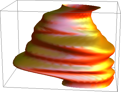
ParametricPlot3D[s[u, v], {u, 0, 1}, {v, 0, 1}, 
                 PlotStyle -> {Orange, Specularity[White, 10]}, Axes -> None, Mesh -> None]

Edit

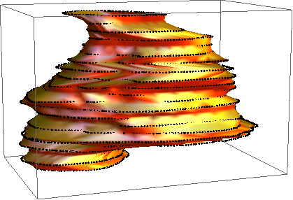
You may toy around with SplineDegree to go from a very smooth surface to a very tight fit for your points. For example with degree -> 1, you get:

s = BSplineFunction[t, SplineDegree -> 1]
Show[{Graphics3D@Point@ptv, 
      ParametricPlot3D[s[u, v], {u, 0, 1}, {v, 0, 1}, 
                       PlotStyle -> {Orange, Specularity[White, 10]}, 
                       Axes ->None,  Mesh -> None]}]