ContourPlot3D wrong plotting result with extra surfaces

Question

Bug introduced after 9.0, persisting through 13.1. Bug report sent on 12/Nov/2022. WRI confirmed the Bug on 18/Nov/2022.

---

I'm trying to plot the following implicit equation in 3D:

Sqrt[x^2+y^2-z^2]+Sqrt[-x^2+y^2+z^2]+Sqrt[x^2-y^2+z^2]=Sqrt[2]

The code I used is:

ContourPlot3D[Sqrt[x^2 + y^2 - z^2] + Sqrt[x^2 - y^2 + z^2] + Sqrt[-x^2 + y^2 + z^2] == Sqrt[2], {x, 0, 1}, {y, 0, 1}, {z, 0, 1}, Mesh -> None, ContourStyle -> {Red, Opacity[0.5]}, MaxRecursion -> 3]

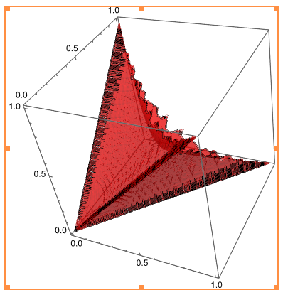
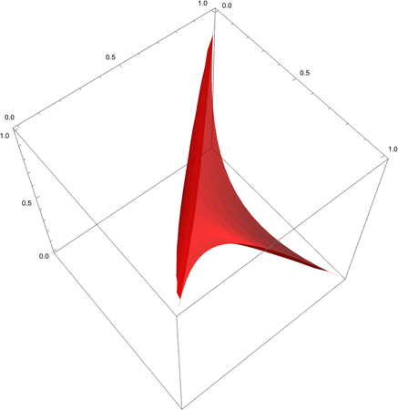
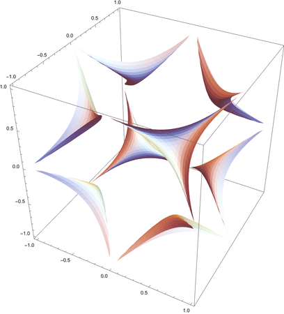
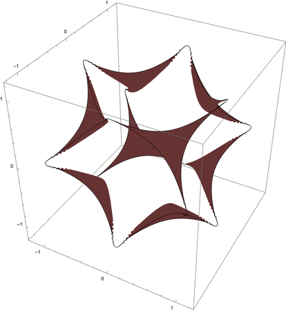
However, the resulting contour plot is weird and wrong - it has three extra surfaces:

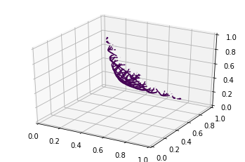
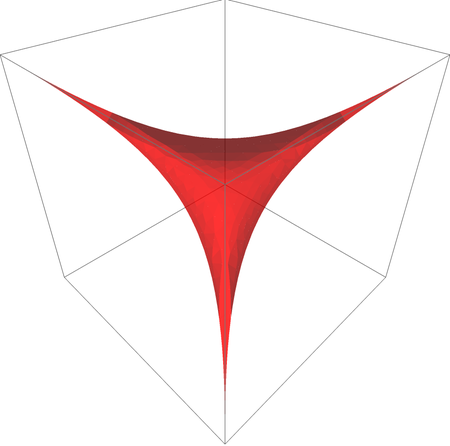
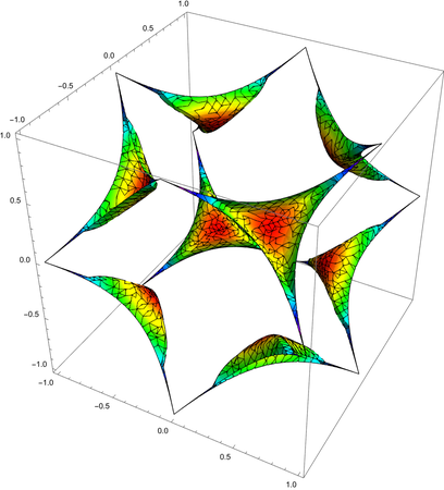
The correct result should be something like the following (made with python)

Could someone help me to identify the issue? Thank you!

Edit: I know the python result is correct because I tried to calculate a few explicit numerical solutions myself.

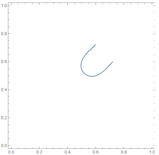
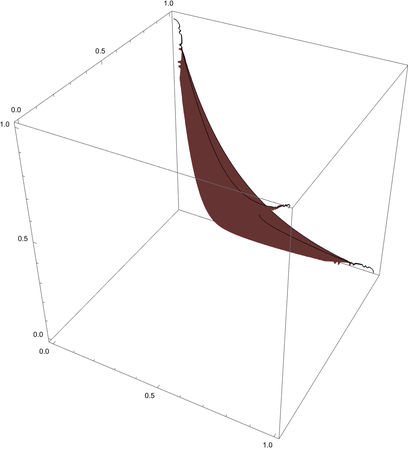
I also tried to plot an x-y intersection when z=0.4 to see how it looks in Mathematica:

k = 0.4;
ContourPlot[
 Sqrt[x^2 + y^2 - k^2] + Sqrt[x^2 - y^2 + k^2] + 
   Sqrt[-x^2 + y^2 + k^2] == Sqrt[2], {x, 0, 1}, {y, 0, 1}, 
 Mesh -> None, Axes -> False]

The python code I used was (which is from this answer)

from mpl_toolkits.mplot3d import axes3d
import matplotlib.pyplot as plt
import numpy as np

def plot_implicit(fn, bbox=(0,1)):
    ''' create a plot of an implicit function
    fn  ...implicit function (plot where fn==0)
    bbox ..the x,y,and z limits of plotted interval'''
    xmin, xmax, ymin, ymax, zmin, zmax = bbox*3
    fig = plt.figure()
    ax = fig.add_subplot(111, projection='3d')
    A = np.linspace(xmin, xmax, 100) # resolution of the contour
    B = np.linspace(xmin, xmax, 15) # number of slices
    A1,A2 = np.meshgrid(A,A) # grid on which the contour is plotted

    for z in B: # plot contours in the XY plane
        X,Y = A1,A2
        Z = fn(X,Y,z)
        cset = ax.contour(X, Y, Z+z, [z], zdir='z')
        # [z] defines the only level to plot for this contour for this value of z

    for y in B: # plot contours in the XZ plane
        X,Z = A1,A2
        Y = fn(X,y,Z)
        cset = ax.contour(X, Y+y, Z, [y], zdir='y')

    for x in B: # plot contours in the YZ plane
        Y,Z = A1,A2
        X = fn(x,Y,Z)
        cset = ax.contour(X+x, Y, Z, [x], zdir='x')

    # must set plot limits because the contour will likely extend
    # way beyond the displayed level.  Otherwise matplotlib extends the plot limits
    # to encompass all values in the contour.
    ax.set_zlim3d(zmin,zmax)
    ax.set_xlim3d(xmin,xmax)
    ax.set_ylim3d(ymin,ymax)

    plt.show()

def surface(x,y,z):
    return np.sqrt(-x*x + y*y + z*z) + np.sqrt(x*x - y*y + z*z) + np.sqrt(x*x + y*y - z*z)- np.sqrt(2)

plot_implicit(surface)

Answer 1

Edit-2

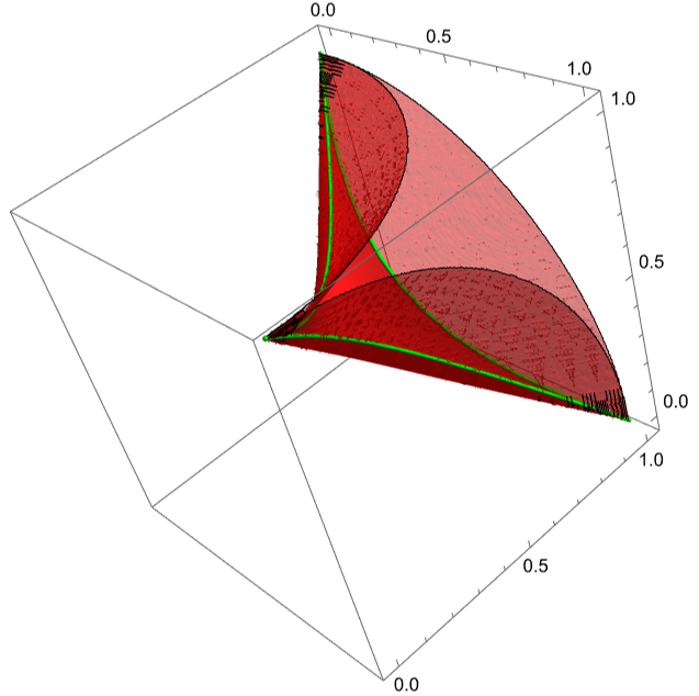
Make the surface smooth.

Clear[sol, expr, plot, reg];
sol = SolveValues[{u^2 == x^2 + y^2 - z^2, v^2 == -x^2 + y^2 + z^2, 
    w^2 == x^2 - y^2 + z^2}, {x, y, z}];
expr = sol // Last
plot = ContourPlot3D[
    u + v + w == Sqrt[2], {u, 0, Sqrt[2]}, {v, 0, Sqrt[2]}, {w, 0, 
     Sqrt[2]}, MaxRecursion -> 4, 
    PlotPoints -> 80] /. {u_Real, v_Real, w_Real} -> expr;
reg = plot // DiscretizeGraphics;
RegionPlot3D[reg, PlotStyle -> {Opacity[.8], Red}, 
 BoundaryStyle -> {Thick, Green}, Axes -> True]

Clear[sol, plot];
sol = SolveValues[{u^2 == x^2 + y^2 - z^2, v^2 == -x^2 + y^2 + z^2, 
    w^2 == x^2 - y^2 + z^2}, {x, y, z}];
plot = ContourPlot3D[
   u + v + w == Sqrt[2], {u, 0, 2}, {v, 0, 2}, {w, 0, 2}, 
   MaxRecursion -> 4, PlotPoints -> 80, Mesh -> None, 
   ContourStyle -> Directive[Opacity[.8], Red]];
Show[(plot /. {u_Real, v_Real, w_Real} -> # & /@ sol), 
 PlotRange -> 1.1]

Edit-1

Use another change of variables.

Clear[sol, expr, reg, meshreg];
sol = SolveValues[{u^2 == x^2 + y^2 - z^2, v^2 == -x^2 + y^2 + z^2, 
    w^2 == x^2 - y^2 + z^2}, {x, y, z}];
expr = sol // Last;
reg = ParametricRegion[{expr, 
    u + v + w == Sqrt[2]}, {{u, 0, 2}, {v, 0, 2}, {w, 0, 2}}];
meshreg = DiscretizeRegion[reg];
Graphics3D[{EdgeForm[], FaceForm[{Red, Opacity[.8]}], meshreg}, 
 ViewPoint -> {1.36, -1.11, 2.89}, Axes -> True]

Clear[sol, regs, meshregs];
sol = SolveValues[{u^2 == x^2 + y^2 - z^2, v^2 == -x^2 + y^2 + z^2, 
    w^2 == x^2 - y^2 + z^2}, {x, y, z}];
regs = ParametricRegion[{#, 
      u + v + w == Sqrt[2]}, {{u, 0, 2}, {v, 0, 2}, {w, 0, 2}}] & /@ 
   sol;
meshregs = DiscretizeRegion /@ regs;
Graphics3D[{EdgeForm[], meshregs}, Axes -> True]

Edit-0

We can change of variables;

Clear[sol];
sol = SolveValues[{u == x^2 + y^2 - z^2, v == -x^2 + y^2 + z^2, 
    w == x^2 - y^2 + z^2}, {x, y, z}];
sol // Last

After that, we at least have two way to do the original plot.

• ParametricRegion+ DiscretizeRegion.

Clear[reg,meshreg];
reg = ParametricRegion[{{Sqrt[u + w]/Sqrt[2], Sqrt[u + v]/Sqrt[2], 
     Sqrt[v + w]/Sqrt[2]}, 
    Sqrt[u] + Sqrt[v] + Sqrt[w] == Sqrt[2]}, {{u, 0, 2}, {v, 0, 
     2}, {w, 0, 2}}];
meshreg = DiscretizeRegion[reg];
RegionPlot3D[meshreg, BoundaryStyle -> None, 
 PlotStyle -> {Red, Opacity[0.8]}, ViewPoint -> {1, 1, 1}]

• ContourPlot3D and change variables.

plot = ContourPlot3D[
   Sqrt[u] + Sqrt[v] + Sqrt[w] == Sqrt[2], {u, 0, 2}, {v, 0, 2}, {w, 
    0, 2}, Mesh -> None, ContourStyle -> White, MaxRecursion -> 2, 
   PlotPoints -> 30];
Show[plot /. {u_Real, v_Real, w_Real} -> {Sqrt[u + w]/Sqrt[2], Sqrt[
    u + v]/Sqrt[2], Sqrt[v + w]/Sqrt[2]}, 
 PlotRange -> {{0, 1}, {0, 1}, {0, 1}}, Lighting -> "ThreePoint"]

• If we remove the restriction 0<=x<=1,0<=y<=1,0<=z<=1, the full surface is

Clear[sol,regs,L];
sol = SolveValues[{u == x^2 + y^2 - z^2, v == -x^2 + y^2 + z^2, 
    w == x^2 - y^2 + z^2}, {x, y, z}];
regs = ParametricRegion[{#, 
      Sqrt[u] + Sqrt[v] + Sqrt[w] == Sqrt[2]}, {{u, 0, 2}, {v, 0, 
       2}, {w, 0, 2}}] & /@ sol;
L = SolveValues[{Sqrt[x^2 + y^2 - z^2] + Sqrt[-x^2 + y^2 + z^2] + 
        Sqrt[x^2 - y^2 + z^2] == Sqrt[2], x == y == z}, {x, y, z}] // 
    First // Norm;
RegionPlot3D[DiscretizeRegion /@ regs // RegionUnion, 
 ColorFunction -> 
  Function[{x, y, z}, 
   Hue[Rescale[Sqrt[x^2 + y^2 + z^2], {L, Sqrt[3]}]]], 
 ColorFunctionScaling -> False, Axes -> True]

Clear[sol,plot];
sol = SolveValues[{u == x^2 + y^2 - z^2, v == -x^2 + y^2 + z^2, 
   w == x^2 - y^2 + z^2}, {x, y, z}]
plot = ContourPlot3D[
   Sqrt[u] + Sqrt[v] + Sqrt[w] == Sqrt[2], {u, 0, 2}, {v, 0, 2}, {w, 
    0, 2}, Mesh -> None, ContourStyle -> White];
Show[plot /. {u_Real, v_Real, w_Real} -> # & /@ sol, PlotRange -> 1.2]

Answer 2

Inspired by cvgmt

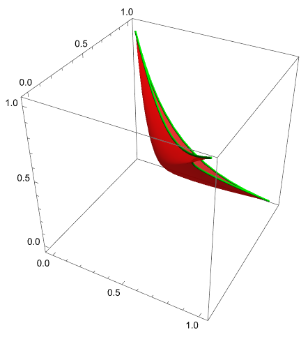
With[{para = Solve[{x^2 + y^2 - z^2, -x^2 + y^2 + z^2, x^2 - y^2 + z^2} == 
  {u, v, Sqrt[2] - u - v}^2, {x, y, z}][[-1, All, 2]]},
 ParametricPlot3D[para, {u, 0, Sqrt[2]}, {v, 0, Sqrt[2] - u}, 
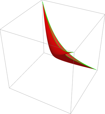
  PlotStyle -> {Opacity[.8], Red}, BoundaryStyle -> Green, Mesh -> None
 ] /. Line -> (Tube[#, 0.006] &)
]

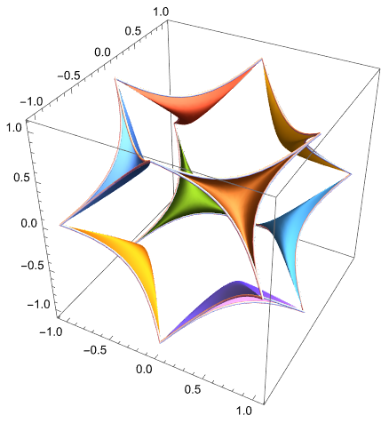
With[{para = Solve[{x^2 + y^2 - z^2, -x^2 + y^2 + z^2, x^2 - y^2 + z^2} == 
  {u, v, Sqrt[2] - u - v}^2, {x, y, z}][[All, All, 2]]},
 ParametricPlot3D[para, {u, 0, Sqrt[2]}, {v, 0, Sqrt[2] - u}, 
   BoundaryStyle -> Automatic, Mesh -> None
   ] /. Line -> (Tube[#, 0.01] &)
 ]

Answer 3

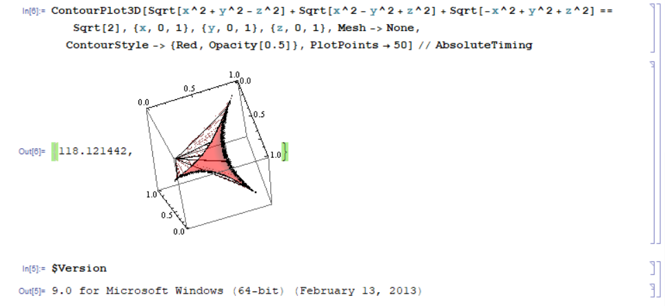
Seems to be a bug introduced after v9. I guess it's essentially the same as this one. In v9, though the quality of plot isn't great, it's correct:

ContourPlot3D[
  Sqrt[x^2 + y^2 - z^2] + Sqrt[x^2 - y^2 + z^2] + Sqrt[-x^2 + y^2 + z^2] == 
   Sqrt[2], {x, 0, 1}, {y, 0, 1}, {z, 0, 1}, Mesh -> None, 
  ContourStyle -> {Red, Opacity[0.5]}, PlotPoints -> 50] // AbsoluteTiming

$Version

Please report it to WRI.

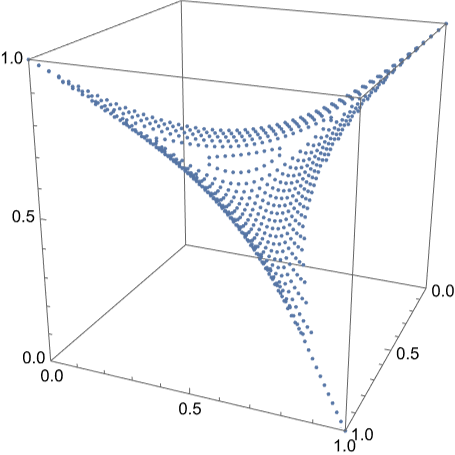
The following is a possible way to get the correct visualization in newer version:

dat = 
   ParallelTable[{x, y, z} /. 
      Solve[Sqrt[x^2 + y^2 - z^2] + Sqrt[x^2 - y^2 + z^2] + Sqrt[-x^2 + y^2 + z^2] ==
          Sqrt[2] // N, z], {x, 0, 1, 1/50}, {y, 0, 1, 1/50}] // 
    Flatten[#, 2] &; // AbsoluteTiming
(* {4.56397, Null} *)
ListPointPlot3D[dat, PlotRange -> {0, 1}, BoxRatios -> {1, 1, 1}]

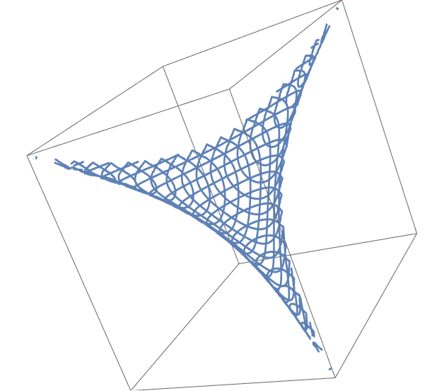
The following is a quick implementation for the idea in the python code:

eq = Sqrt[x^2 + y^2 - z^2] + Sqrt[x^2 - y^2 + z^2] + Sqrt[-x^2 + y^2 + z^2] == 
   Sqrt[2];

{Table[Normal@ContourPlot[eq // Evaluate, {x, 0, 1}, {z, 0, 1}] /. 
     Line[a_] :> Line[{#, y, #2} & @@@ a], {y, 0, 1, 1/25}], 
   Table[Normal@ContourPlot[eq // Evaluate, {y, 0, 1}, {z, 0, 1}] /. 
     Line[a_] :> Line[{x, #, #2} & @@@ a], {x, 0, 1, 1/25}], 
   Table[Normal@ContourPlot[eq // Evaluate, {x, 0, 1}, {y, 0, 1}] /. 
     Line[a_] :> Line[{#, #2, z} & @@@ a], {z, 0, 1, 1/25}]} /. 
  Graphics -> Graphics3D // Show[#, PlotRange -> All] &

Sadly I've no idea how to get the desired surface.

---

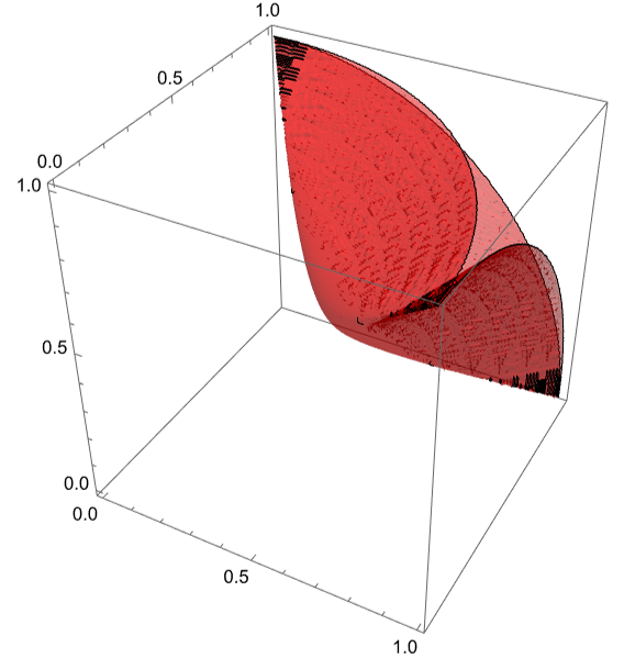
I just realized something so funny that it's worth mentioning here. The bug can be partly circumvented in the following ridiculous manner:

eq = Sqrt[x^2 + y^2 - z^2] + Sqrt[x^2 - y^2 + z^2] + Sqrt[-x^2 + y^2 + z^2] == 
   Sqrt[2];

lhs = Subtract @@ eq;

pic = ContourPlot3D[0 == lhs, {x, 0, 1}, {y, 0, 1}, {z, 0, 1}, Mesh -> None, 
  ContourStyle -> {Red, Opacity[0.5]}, MaxRecursion -> 3]

See what I've done? I've only made a trivial transform on eq i.e. re-write eq to the equivalent 0 == lhs. (An alternatve is -lhs == 0, BTW. )

Compare with the graphic in chyanog's answer:

With[{para = 
    Solve[{x^2 + y^2 - z^2, -x^2 + y^2 + z^2, 
        x^2 - y^2 + z^2} == {u, v, Sqrt[2] - u - v}^2, {x, y, z}][[-1, All, 2]]}, 
  ParametricPlot3D[para, {u, 0, Sqrt[2]}, {v, 0, Sqrt[2] - u}, 
    PlotStyle -> {Opacity[.8], Red}, BoundaryStyle -> Green, Mesh -> None] /. 
   Line -> (Tube[#, 0.006] &)]~Show~pic

We see this new surface does contain the true solution, but also involves fake solution.