8
$\begingroup$

Calculation of stress in two dimensions is covered in this post by the helpful user21. I am now trying to work in three dimensions. For this we need a stress operator which I have taken from Help.

ClearAll[stressOperator, u, v, w, x, y, z, Y, ν]; 
stressOperator[
  Y_, ν_] := {Inactive[
     Div][{{0, 0, -((Y*ν)/((1 - 2*ν)*(1 + ν)))}, {0, 0, 
       0}, {-Y/(2*(1 + ν)), 0, 0}}.Inactive[Grad][
      w[x, y, z], {x, y, z}], {x, y, z}] + 
   Inactive[
     Div][{{0, -((Y*ν)/((1 - 2*ν)*(1 + ν))), 
       0}, {-Y/(2*(1 + ν)), 0, 0}, {0, 0, 0}}.Inactive[Grad][
      v[x, y, z], {x, y, z}], {x, y, z}] + 
   Inactive[
     Div][{{-((Y*(1 - ν))/((1 - 2*ν)*(1 + ν))), 0, 
       0}, {0, -Y/(2*(1 + ν)), 0}, {0, 
       0, -Y/(2*(1 + ν))}}.Inactive[Grad][
      u[x, y, z], {x, y, z}], {x, y, z}], 
  Inactive[Div][{{0, 0, 0}, {0, 
       0, -((Y*ν)/((1 - 
              2*ν)*(1 + ν)))}, {0, -Y/(2*(1 + ν)), 
       0}}.Inactive[Grad][w[x, y, z], {x, y, z}], {x, y, z}] + 
   Inactive[
     Div][{{0, -Y/(2*(1 + ν)), 
       0}, {-((Y*ν)/((1 - 2*ν)*(1 + ν))), 0, 0}, {0, 0, 
       0}}.Inactive[Grad][u[x, y, z], {x, y, z}], {x, y, z}] + 
   Inactive[
     Div][{{-Y/(2*(1 + ν)), 0, 
       0}, {0, -((Y*(1 - ν))/((1 - 2*ν)*(1 + ν))), 0}, {0,
        0, -Y/(2*(1 + ν))}}.Inactive[Grad][
      v[x, y, z], {x, y, z}], {x, y, z}], 
  Inactive[Div][{{0, 0, 0}, {0, 
       0, -Y/(2*(1 + ν))}, {0, -((Y*ν)/((1 - 
              2*ν)*(1 + ν))), 0}}.Inactive[Grad][
      v[x, y, z], {x, y, z}], {x, y, z}] + 
   Inactive[
     Div][{{0, 0, -Y/(2*(1 + ν))}, {0, 0, 
       0}, {-((Y*ν)/((1 - 2*ν)*(1 + ν))), 0, 0}}.Inactive[
       Grad][u[x, y, z], {x, y, z}], {x, y, z}] + 
   Inactive[
     Div][{{-Y/(2*(1 + ν)), 0, 0}, {0, -Y/(2*(1 + ν)), 0}, {0,
        0, -((Y*(1 - ν))/((1 - 2*ν)*(1 + ν)))}}.Inactive[
       Grad][w[x, y, z], {x, y, z}], {x, y, z}]}

Here is an example of the application.

Needs["NDSolve`FEM`"];

Len = 1;  (*length *)
ht = 0.125; (* height *)
wd = 0.5; (* width *)
materialParameters = {Y -> 10^3, ν -> 33/100};
ss = 1;(*Shear stress on beam end*)
reg = Cuboid[{0, -wd/2, 0}, {Len, wd/2, ht}];
mesh = ToElementMesh[reg];
mesh["Wireframe"]

Mathematica graphics

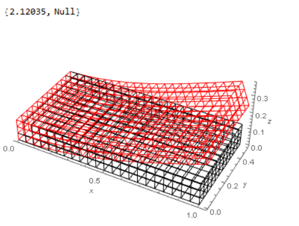
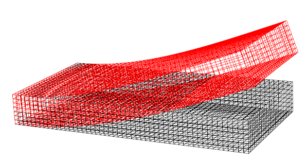
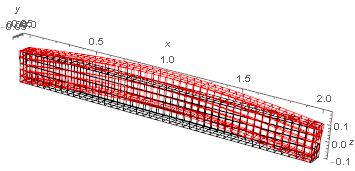
The problem is a thick beam clamped at one end with a shear stress on the other. To solve for the deflections I use

{uif, vif, wif} = NDSolveValue[{
     stressOperator[Y, ν] == {0, 0, NeumannValue[ss, x == Len]},
     DirichletCondition[u[x, y, z] == 0, x == 0],
     DirichletCondition[v[x, y, z] == 0, x == 0],
     DirichletCondition[w[x, y, z] == 0, x == 0]
     } /. materialParameters, {u, v, w}, {x, y, z} ∈ mesh];

dmesh = ElementMeshDeformation[mesh, {uif, vif, wif}, 
   "ScalingFactor" -> 1];
Show[{mesh["Wireframe"], 
  dmesh["Wireframe"[
    "ElementMeshDirective" -> Directive[EdgeForm[Red], FaceForm[]]]]}]
Mathematica graphics

All this is working well. Now I would like to find stresses and vonMises stress. I began to look at the equations but thought I would be lazy and see if anyone has done this already. How do I get from the displacements to the stress? Thanks for your efforts if you have done this.

Edit - a module for stresses

I examined the answer from Mauricio Lobos (thank you) but could not put together a simple module for calculating stress. I did manages to put one together based on extending the 2D example to 3D. Here it is

 ClearAll[stress3D];
    stress3D::usage = 
      "stress3D[{u,v,w},{Y,ν}] determines interpolation functions for \
    stress from the interpolation functions {u,v,w} for displacement in \
    each direction. {Y,ν} are the modulus of elasticity and Poission  \
    ratio.
      The output is a list of the three normal stress components, three \
    shear stresses and finally the von Mises stress";
    stress3D[{uif_InterpolatingFunction, vif_InterpolatingFunction, 
       wif_InterpolatingFunction}, {Y_, ν_}] :=
     Block[{dd, df, mesh, coords, dv, ux, uy, uz, vx, vy, vz, wx, wy, wz, 
       gxy, gxz, gyz, c1, c2, c3, sxx, syy, szz, sxy, syz, szx, vonM},
      dd = Outer[(D[#1[x, y, z], #2]) &, {uif, vif, wif}, {x, y, z}];(* 
      make derivative interpolation functions *)
      df = Table[
        Function[{x, y, z}, Evaluate[dd[[i, j]]]], {i, 3}, {j, 3}]; (* 
      make functions for each derivative *)

       mesh = uif["Coordinates"][[1]]; (* extract coordinates from mesh *)


      coords = mesh["Coordinates"];

      dv = Table[df[[i, j]] @@@ coords, {i, 3}, {j, 3}]; (* 
      get values of derivatives at each node *)

      ux = dv[[1, 1]]; (* extract individual strain components *)
      uy = dv[[1, 2]];
      uz = dv[[1, 3]];
      vx = dv[[2, 1]];
      vy = dv[[2, 2]];
      vz = dv[[2, 3]];
      wx = dv[[3, 1]];
      wy = dv[[3, 2]];
      wz = dv[[3, 3]];

      gxy = (uy + vx); (* shear strains *)
      gxz = (uz + wx);
      gyz = (vz + wy);


      c1 = Y/((1 - 2 ν) (1 + ν));(* Constitutive constants *)
      c2 = (1 - ν);
      c3 = Y/(2 (1 + ν));
      sxx = c1 ( c2 ux + ν vy + ν wz); (*stresses *)
      syy = c1 ( ν ux + c2 vy + ν wz);
      szz = c1 ( ν ux + ν vy + c2 wz);
      sxy = c3 gxy; (* shear stresses *)
      syz = c3 gyz;
      szx = c3 gxz;
      vonM = Sqrt[
       1/2 ((sxx - syy)^2 + (syy - szz)^2 + (szz - sxx)^2 + 
          6 (sxy^2 + syz^2 + szx^2))];
      {
       ElementMeshInterpolation[{mesh}, sxx],
       ElementMeshInterpolation[{mesh}, syy],
       ElementMeshInterpolation[{mesh}, szz],
       ElementMeshInterpolation[{mesh}, sxy],
       ElementMeshInterpolation[{mesh}, syz],
       ElementMeshInterpolation[{mesh}, szx],
       ElementMeshInterpolation[{mesh}, vonM]
       } 
      ]

This produces the normal stresses and the shear stress (6 interpolating functions) and also the von Mises stress (last interpolating function).

Continuing with the example the stresses are calculated by

{sxx, syy, szz, sxy, syz, szx, vM} = 
  stress3D[{uif, vif, wif}, {Y, ν} /. materialParameters];

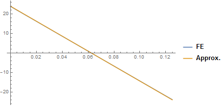
The results can be checked by using the approximate engineering theory for the a beam. The force at the end of the beam and the second moment of area are given by

 force = ss ht wd;
    I2 = 1/12 wd ht^3;

The shear stress at one section can be calculated as

With[{x = 0.5},
 Plot[{sxx[x, 0, z], (ht/2 - z) force (Len - x)/I2}, {z, 0, ht}]
 ]
Mathematica graphics

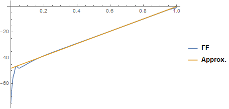
Which agrees well. The shear stress along the beam can be calculated from

Plot[{sxx[x, 0, ht], -(ht /(2 I2)) force (Len - x),}, {x, 0, Len}, 
 PlotLegends -> LineLegend[{"FE", "Approx."}]]
Mathematica graphics

Again this agrees well except at the root where the FE is more correct. The shear stress in the z direction on the cross-section is given by

With[{x = 0.5},
 Plot[{szx[x, 0, z], (ss wd ht)/(2 I2) (ht^2/4 - (z - ht/2)^2)}, {z, 
   0, ht}, PlotLegends -> LineLegend[{"FE", "Approx."}]]
 ]
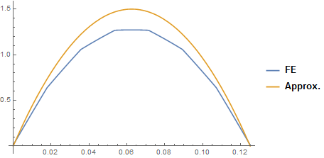
Mathematica graphics

Which is slightly off. This may be because the approximate theory is only good for cross-sections which are small compared to the length. Also, we could do with more grid. Finally looking at the shear stress where it is applied to the end of the beam gives.

Plot[{szx[Len, 0, z], ss}, {z, 0, ht}, PlotRange -> All, 
 PlotLegends -> LineLegend[{"FE", "Approx."}]]
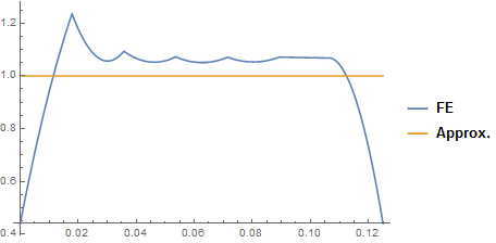
Mathematica graphics

Again this is a bit disappointing since the shear stress is applied equally over the end. Again this may be due to a poor mesh.

Overall the results look reasonable. I hope you find the module for calculating stress useful. Let me know if there are problems.

$\endgroup$

1 Answer 1

10
$\begingroup$

Take a look at this post

https://mathematica.stackexchange.com/a/132278/24710


Short answer:

you can get the 3D stresses by using the 3D Hooke's law, i.e., $\sigma_{ij} = C_{ijkl} \varepsilon_{kl}$ and using the interpolation functions from the FEM solution. If your stiffness tensor is symmetric in $kl$ and isotropic, then you can immediatly use $\sigma_{ij} = C_{ijkl} (\partial{u_k}/\partial x_{l})$. You can then compute the pressure part of the stress $\sigma^°=(\sigma_{kk}/3) I$ and then the deviatoric part $\sigma' = \sigma - \sigma^°$. The Frobenius norm of the stress deviator is used in order to computed the von Mises stress $\sigma_{vM} = \sqrt{3/2} ||\sigma' ||$, where the Frobenius norm is defined as $||A|| = \sqrt{A \cdot A} = \sqrt{A_{ij}A_{ij}}$. If you want to check initiation of plastic deformation triggered at a yield stress $\sigma_y$, then check $\sigma_{vM} \leq \sigma_y$.


Long answer and example

Here, just an extract of post https://mathematica.stackexchange.com/a/132278/24710 . Consider a rectangle with lengths L1, L2 and L3 and loaded with a normal force density per unit area qA. Young's modulus Em and Poissons ratio nu are also assumed as

(*Geometry-in m*)
L1 = 2;
L2 = 0.1;
L3 = 0.2;
(*Force and densities-in N*)
F = 10;
qA = F/(L1*L2);
(*Material parameters*)
Em = 2.1*10^9;(*Young's modulus*)
nu = 0.3;(*Poisson's ration*)

Consider this 3D FEM solution

(*FEM solution*)
Needs["NDSolve`FEM`"]
(******************************)
(*Region definition*)
reg = Cuboid[{0, -L2/2, -L3/2}, {L1, L2/2, L3/2}];
(******************************)
(*Isotropic material stiffness-fourth-order tensor*)
(*Identities*)
I2 = IdentityMatrix@3;
IdI = TensorProduct[I2, I2];
I4 = TensorTranspose[IdI, {1, 3, 2, 4}];
IS = (I4 + TensorTranspose[I4, {1, 2, 4, 3}])/2;
(*Isotropic projectors*)
P1 = 1/3*IdI;
P2 = IS - P1;
(*Isotropic stiffness*)
Ciso = l1*P1 + l2*P2;
l1 = 3*Km;
l2 = 2*Gm;
Km = 1/3*Em/(1 - 2*nu);
Gm = 1/2*Em/(1 + nu);
(******************************)
(*Equations*)
eq = Table[
   Inactive[Div][
     Ciso[[i, ;; , 1, ;;]].Inactive[Grad][u[x, y, z], {x, y, z}], {x, 
      y, z}] + 
    Inactive[Div][
     Ciso[[i, ;; , 2, ;;]].Inactive[Grad][v[x, y, z], {x, y, z}], {x, 
      y, z}] + 
    Inactive[Div][
     Ciso[[i, ;; , 3, ;;]].Inactive[Grad][w[x, y, z], {x, y, z}], {x, 
      y, z}], {i, 3}];
(******************************)
(*BCs*)
(*Dirichlet*)
bcD = {DirichletCondition[{u[x, y, z] == 0, v[x, y, z] == 0, 
     w[x, y, z] == 0}, x == 0 && z == 0], 
   DirichletCondition[{v[x, y, z] == 0, w[x, y, z] == 0}, 
    x == L1 && z == 0]};
(*Neumann*)
bcN = {0, 0, NeumannValue[-qA, z == -L3/2]};
(******************************)
(*Solution*)
{usol, vsol, wsol} = 
   NDSolveValue[{eq == bcN, bcD}, {u, v, w}, Element[{x, y, z}, reg], 
    Method -> {"PDEDiscretization" -> {"FiniteElement", 
        "MeshOptions" -> {"MaxCellMeasure" -> 0.0001, 
          "MeshOrder" -> 2}}}]; // AbsoluteTiming

If you want to see the deformed body, use

mesh = usol["ElementMesh"];
Show[{
  mesh["Wireframe"]
  , ElementMeshDeformation[mesh, {usol, vsol, wsol}, 
    "ScalingFactor" -> 10^4][
   "Wireframe"[
    "ElementMeshDirective" -> Directive[EdgeForm[Red], FaceForm[]]]]
  }, Axes -> True, AxesLabel -> {x, y, z}]

enter image description here

Now you can use the 3D solution in order to build up your Hooke's law with the isotropic stiffness

uv[x_, y_, z_] := {usol[x, y, z], vsol[x, y, z], wsol[x, y, z]}
eps[xs_, ys_, zs_] := D[uv[x, y, z], {{x, y, z}, 1}] /. {x -> xs, y -> ys, z -> zs}
(*linear map of second order tensor B over fourth-order tensor A*)
lm[A_, B_] := TensorContract[TensorProduct[A, B], {{3, 5}, {4, 6}}]
(*Hooke's law*)
sig[x_, y_, z_] := lm[Ciso, eps[x, y, z]]

Based on the defined stress you can compute what you want

(*Stress deviator and von Mises stress*)
sigd[x_, y_, z_] := sig[x, y, z] - Tr[sig[x, y, z]]/3*IdentityMatrix[3];
svm[x_, y_, z_] := Sqrt[3/2]*Norm[sigd[x, y, z], "Frobenius"];

Example:

sig[L1/2, 0, 0]
svm[L1/2, 0, 0]

{{-1.78038*10^-9, 2.3347*10^-10, -0.146191}, {2.3347*10^-10, -1.29736*10^-9,-6.32158*10^-10}, {-0.146191, -6.32158*10^-10, -25.}}

25.0013


EDIT

Consider now this code for the generation of the FEM solution

Needs["NDSolve`FEM`"];
(*************************************)
(*Geometry-in m*)
L1 = 1;
L2 = 0.5;
L3 = 0.125;
(*Surface force density in N/m^2*)
sF = 1;
(*Material parameters*)
Em = 10^3;(*Young's modulus in N/m^2*)
nu = 33/100;(*Poisson's ration - dimensionless*)
(*************************************)
(*Region*)
reg = Cuboid[{0, 0, 0}, {L1, L2, L3}];
(*BCs*)
(*Dirichlet*)
bcD = {
   DirichletCondition[{u[x, y, z] == 0, v[x, y, z] == 0, 
     w[x, y, z] == 0}, x == 0]
   };
(*Neumann*)
bcN = {0, 0, NeumannValue[sF, x == L1]};
(*Homogeneous material stiffness*)
(*************************************)
(*Isotropic material stiffness-fourth-order tensor*)
(*Identities*)
I2 = IdentityMatrix@3;
IdI = TensorProduct[I2, I2];
I4 = TensorTranspose[IdI, {1, 3, 2, 4}];
IS = (I4 + TensorTranspose[I4, {1, 2, 4, 3}])/2;
(*Isotropic projectors*)
P1 = 1/3*IdI;
P2 = IS - P1;
(*Isotropic stiffness*)
stiff = l1*P1 + l2*P2;
l1 = 3*Km;
l2 = 2*Gm;
Km = 1/3*Em/(1 - 2*nu);
Gm = 1/2*Em/(1 + nu);
(*************************************)
eq = Table[
   Inactive[Div][
     stiff[[i, ;; , 1, ;;]].Inactive[Grad][u[x, y, z], {x, y, z}], {x,
       y, z}] + 
    Inactive[Div][
     stiff[[i, ;; , 2, ;;]].Inactive[Grad][v[x, y, z], {x, y, z}], {x,
       y, z}] + 
    Inactive[Div][
     stiff[[i, ;; , 3, ;;]].Inactive[Grad][w[x, y, z], {x, y, z}], {x,
       y, z}], {i, 3}];
(*************************************)
{u21, u22, u23} = 
   NDSolveValue[{-eq == bcN, bcD}, {u, v, w}, Element[{x, y, z}, reg],
     Method -> {"PDEDiscretization" -> {"FiniteElement", 
        "MeshOptions" -> {"MaxCellMeasure" -> 0.0001, 
          "MeshOrder" -> 2}}}]; // AbsoluteTiming
(*************************************)
mesh = u21["ElementMesh"];
Show[{mesh["Wireframe"], 
  ElementMeshDeformation[mesh, {u21, u22, u23}, 
    "ScalingFactor" -> 10^0][
   "Wireframe"[
    "ElementMeshDirective" -> Directive[EdgeForm[Red], FaceForm[]]]]},
  Axes -> True, AxesLabel -> {x, y, z}]

enter image description here

The following module, based on the description given above, returns the Cauchy-stress as a function for input interpolation functions u1, u2 and u3 and homogeneous stiffness tensor stiff (given as fourth-order tensor)

lm[A_, B_] := TensorContract[TensorProduct[A, B], {{3, 5}, {4, 6}}]
stress3D[{u1_, u2_, u3_}, stiff_, {x1_, x2_, x3_}] := Module[
   {u, gu, xd1, xd2, xd3},
   u = Function[{x1, x2, x3}, {u1[x1, x2, x3], u2[x1, x2, x3], 
      u3[x1, x2, x3]}];
   gu = Function[{x1, x2, x3}, 
     D[u[xd1, xd2, xd3], {{xd1, xd2, xd3}, 1}] /. {xd1 -> x1, 
       xd2 -> x2, xd3 -> x3}];
   Function[{x1, x2, x3}, lm[stiff, gu[x1, x2, x3]]]
   ];

I will get the stress for your problem and save the complete stress tensor in temp

temp = stress3D[{u21, u22, u23}, stiff, {x1, x2, x3}];
GraphicsRow[{
  Plot[temp[L1/2, L2/2, z][[1, 1]], {z, 0, L3}, 
   PlotLabel -> "\!\(\*SubscriptBox[\(σ\), \(xx\)]\) at x=L1/2"]
  , Plot[temp[x, L2/2, L3][[1, 1]], {x, 0, L1}, 
   PlotLabel -> "\!\(\*SubscriptBox[\(σ\), \(xx\)]\) at z=L3"]
  , Plot[temp[L1/2, L2/2, z][[3, 1]], {z, 0, L3}, 
   PlotLabel -> "\!\(\*SubscriptBox[\(σ\), \(zx\)]\) at x=L1/2"]
  , Plot[temp[L1, L2/2, z][[3, 1]], {z, 0, L3}, 
   PlotLabel -> "\!\(\*SubscriptBox[\(σ\), \(zx\)]\) at x=L1"]
  }
 , ImageSize -> 1000
 ]

enter image description here

I used quadratic elemets for a continuous stress variation and my origin is a (0,0,0). Based on the description given above, you can compute whatever you want with the stress tensor, e.g., the von-Mises stress and other quantities.

I would like to note, that, from a mechanical point of view, this specific problem should NOT be treated as a beam (L2 and L3 should be significantly smaller than L1). Also, the deformations seems to be quite large, such that the linearized theory (used in this example), is not appropriate. Just as a remark.

$\endgroup$
3
  • $\begingroup$ Just a note to say thank you. Can you put together your solution for stresses in a module so that it can be used on different problems? I have done this for my question and it would be good to check what I have done against your method. $\endgroup$
    – Hugh
    Commented Apr 11, 2017 at 18:28
  • 1
    $\begingroup$ Ok, I will do it in the next days. It can take a while, I am traveling right now. $\endgroup$ Commented Apr 11, 2017 at 18:58
  • $\begingroup$ @Hugh take a look at my edit, may be that helps you. $\endgroup$ Commented Apr 14, 2017 at 14:21

Your Answer

By clicking “Post Your Answer”, you agree to our terms of service and acknowledge you have read our privacy policy.

Not the answer you're looking for? Browse other questions tagged or ask your own question.