How to improve quality of NeumannValue boundary conditions for stress calculations

Question

When doing stress calculations forces are applied to a boundary of a region. Here I am applying the forces over an interval but the stress resolution is poor near the edge of the interval. Can this be improved?

For this minimum working example I am applying the stress to one side of a bar and holding the bar on the opposite side. Here are some starting modules that will be used subsequently.

Needs["NDSolve`FEM`"]

ClearAll[planeStress]; 
planeStress[
  Y_, ν_] := {Inactive[
     Div][{{-(Y/(1 - ν^2)), 
       0}, {0, -((Y*(1 - ν))/(2*(1 - ν^2)))}} . 
     Inactive[Grad][u[x, y], {x, y}], {x, y}] + 
       Inactive[
     Div][{{0, -((Y*ν)/(1 - ν^2))}, {-((Y*(1 - ν))/(2*(1 \
- ν^2))), 0}} . Inactive[Grad][v[x, y], {x, y}], {x, y}], 
     Inactive[
     Div][{{0, -((Y*(1 - ν))/(2*(1 - ν^2)))}, {-((Y*ν)/(1 \
- ν^2)), 0}} . Inactive[Grad][u[x, y], {x, y}], {x, y}] + 
       Inactive[
     Div][{{-((Y*(1 - ν))/(2*(1 - ν^2))), 
       0}, {0, -(Y/(1 - ν^2))}} . 
     Inactive[Grad][v[x, y], {x, y}], {x, y}]}

ClearAll[stress2D]
stress2D[{uif_InterpolatingFunction, 
   vif_InterpolatingFunction}, {Y_, ν_}] :=
 Block[{fac, dd, df, mesh, coords, dv, ux, uy, vx, vy, ex, ey, gxy, 
   sxx, syy, sxy},
  dd = Outer[(D[#1[x, y], #2]) &, {uif, vif}, {x, y}];
  fac = Y/(1 - ν^2)*{{1, ν, 0}, {ν, 1, 0}, {0, 
      0, (1 - ν)/2}};
  df = Table[Function[{x, y}, Evaluate[dd[[i, j]]]], {i, 2}, {j, 2}];
  (*the coordinates from the ElementMesh*)
  mesh = uif["Coordinates"][[1]];
  coords = mesh["Coordinates"];
  dv = Table[df[[i, j]] @@@ coords, {i, 2}, {j, 2}];
  ux = dv[[1, 1]];
  uy = dv[[1, 2]];
  vx = dv[[2, 1]];
  vy = dv[[2, 2]];
  ex = ux;
  ey = vy;
  gxy = (uy + vx);
  sxx = fac[[1, 1]]*ex + fac[[1, 2]]*ey;
  syy = fac[[2, 1]]*ex + fac[[2, 2]]*ey;
  sxy = fac[[3, 3]]*gxy;
  {ElementMeshInterpolation[{mesh}, sxx],
   ElementMeshInterpolation[{mesh}, syy],
   ElementMeshInterpolation[{mesh}, sxy]
       }]


ClearAll[solveFE];
solveFE[mesh_, col_, n_] := 
 Module[{uif, vif, sxx, syy, sxy, nodes, top, syypts, p1, p2},
  {uif, vif} = 
   NDSolveValue[{planeStress[Y, ν] == {0, 
       NeumannValue[-stress, -(sL/2) <= x <= sL/2 && y == h]},

     DirichletCondition[v[x, y] == 0, -(cL/2) <= x <= cL/2 && y == 0], 

     DirichletCondition[u[x, y] == 0, x == 0 && y == 0]},
         {u, v}, Element[{x, y}, mesh]];
  {sxx, syy, sxy} = stress2D[{uif, vif}, {Y, ν}];
  nodes = mesh["Coordinates"];
  top = Select[nodes, #[[2]] == h &];
  syypts = {#[[1]], syy[#[[1]], #[[2]]]} & /@ top;
  Show[Plot[syy[x, h], {x, -L/2, L/2}, PlotRange -> {{-sL, sL}, All}, 
    PlotStyle -> col,
    PlotLegends -> LineLegend[{col}, {n}]],
   Graphics[{Point[syypts], Line[{{-sL/2, -stress}, {sL/2, -stress}}]}]
   ]
  ]

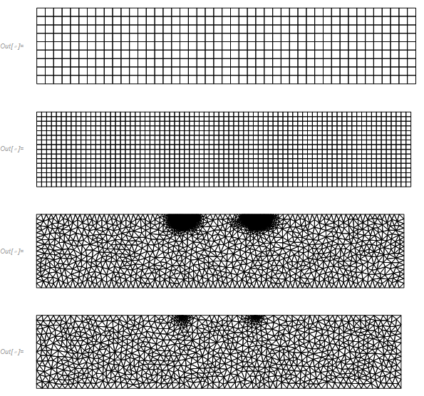
Now we make four meshes in an attempt to accurately represent the interval over which the force is applied. The first mesh is the default, the second a finer mesh everywhere, the third refinement at the ends of the interval and the final mesh considerable refinement with a node at the end of the interval.

L = 1; (* Length *)
h = 0.2; (* Height *)
Y = 20 10^10;(* Modulus of elasticity *)
ν = 33/100; (* Poission ratio *)
sL = L/5; (* Interval for applied force *)
cL = L/5; (* Interval for support *)
stress = 100;
(* Default mesh *)
mesh1 = ToElementMesh[Rectangle[{-(L/2), 0}, {L/2, h}]];

(* mesh with finer resolution *)
gls = Min[1/10 { L, h}]; (* grid lenght scale *)
mesh2 = ToElementMesh[Rectangle[{-(L/2), 0}, {L/2, h}], 
   MaxCellMeasure -> (Sqrt[3]/4)*gls^2];

(* mesh enhanced around ends of force interval *)
ref = gls/10;
cf = Compile[{{c, _Real, 2}, {a, _Real, 0}},
   Block[{com, c1 = {-sL/2, h}, c2 = {sL/2, h}},
    com = Total[c]/3;
    If[(Norm[com - c1] < h/5 || Norm[com - c2] < h/5) && 
      a > (Sqrt[3]/4) ref^2, True, False]
    ]];
mesh3 = ToElementMesh[Rectangle[{-(L/2), 0}, {L/2, h}], 
   MaxCellMeasure -> (Sqrt[3]/4)*gls^2, MeshRefinementFunction -> cf];

(* mesh much enhanced around ends of force interval with node at each \
end *)  
 r = h/5; (* distance from end of interval *)
cf = Compile[{{c, _Real, 2}, {a, _Real, 0}},
   Block[{com, c1 = {-sL/2, h}, c2 = {sL/2, h}, d1, d2},
    com = Total[c]/3;
    d1 = Norm[com - c1];
    d2 = Norm[com - c2];
    Which[
     d1 < r && a > (Sqrt[3]/4) (gls/100 + d1/r (gls - gls/100))^2, 
     True,
     d2 < r && a > (Sqrt[3]/4) (gls/100 + d2/r (gls - gls/100))^2, 
     True,
     True, False
     ]
    ]];
cc = {{-L/2, 0}, {L/2, 0}, {L/2, h}, {sL/2, h}, {-sL/2, h}, {-L/2, h}};
bmesh = ToBoundaryMesh[
   "Coordinates" -> cc,
   "BoundaryElements" -> {LineElement[{{1, 2}, {2, 3}, {3, 4}, {4, 
        5}, {5, 6}, {6, 1}}]},
   "MaxBoundaryCellMeasure" -> gls];
mesh4 = ToElementMesh[bmesh, MaxCellMeasure -> (Sqrt[3]/4)*gls^2, 
   MeshRefinementFunction -> cf];

The meshes look as follows

mesh1["Wireframe"]
mesh2["Wireframe"]
mesh3["Wireframe"]
mesh4["Wireframe"]

Now we solve using each mesh and look at the stresses along the top of the bar.

p1 = solveFE[mesh1, Orange, 1];
p2 = solveFE[mesh2, Purple, 2];
p3 = solveFE[mesh3, Brown, 3];
p4 = solveFE[mesh4, Green, 4];
Column[{p1, p2, p3, p4}]
s = 0.2;
Show[p1, p2, p3, p4, PlotRange -> {{(1 - s) sL/2, (1 + s) sL/2}, All}]

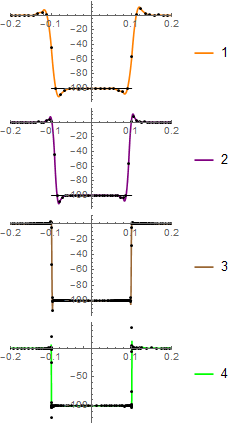
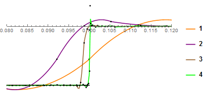
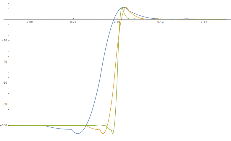
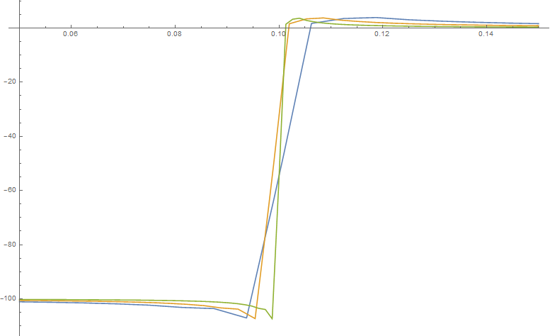
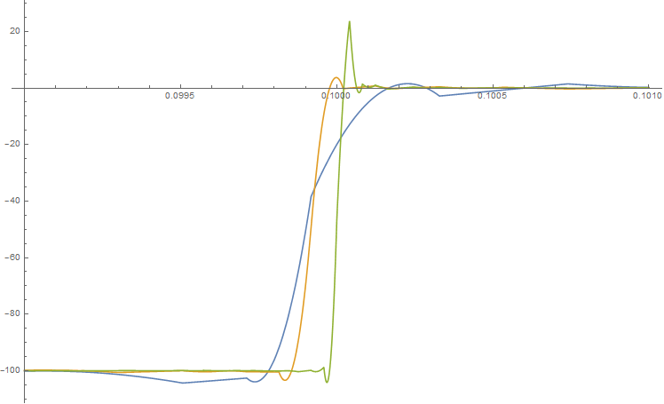
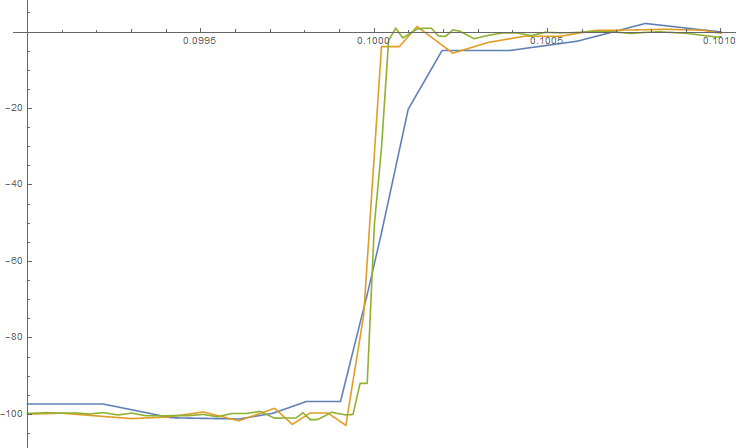
Each mesh is an improvement on the previous. However, all the meshes have considerable overshoot and give stresses outside the interval. Can this be improved or is it an inevitable result of the interpolation? Things are even worse if one looks at the stresses on the support under the bar.

Answer 1

I have done some thinking and note the following. The stress is approximately proportional to the derivative of the displacement. Further the displacements are continuous but the stress is discontinuous at the ends of the interval along which it is applied. With the default MeshOrder of 2 the solution and its derivative are continuous. Thus it cannot represent a discontinuous function. However, if I use MeshOrder 1 then the displacements will be continuous but the derivative can be discontinuous. This could be what I need. However it comes with the penalty of needing more elements.

As an example I tried to make three meshes with rectangular elements first with 2nd order meshes and then with 1st order meshes. I used twice the resolution with 1st order meshes. This is the code

ClearAll[solve];
solve[mo_, gls_] := Module[{mesh},
  mesh = ToElementMesh[Rectangle[{-(L/2), 0}, {L/2, h}], 
    MaxCellMeasure -> (Sqrt[3]/4)*gls^2, "MeshOrder" -> mo];
  {uif, vif} = 
   NDSolveValue[{planeStress[Y, ν] == {0, 
       NeumannValue[-stress, -(sL/2) <= x <= sL/2 && y == h]}, 
     DirichletCondition[v[x, y] == 0, -(cL/2) <= x <= cL/2 && y == 0],
      DirichletCondition[u[x, y] == 0, x == 0 && y == 0]}, {u, v}, 
    Element[{x, y}, mesh]];
  {sxx, syy, sxy} = stress2D[{uif, vif}, {Y, ν}];
  {uif, vif, sxx, syy, sxy}
  ]

Here we make three meshes with 2nd order elements

ClearAll[sol];
mr = {10, 20, 50};
Do[sol[n] = solve[2, h/n];, {n, mr}]

a = 0.5;
Plot[Evaluate[Table[sol[n][[4]][x, h], {n, mr}]],
 {x, (1 - a) sL/2, (1 + a) sL/2},
 PlotRange -> All]

Note the overshoot of about 10%.

Now with first order meshes.

mr2 = {21, 40, 100};
Do[sol[n] = solve[1, h/n];, {n, mr2}]

a = 0.5;
Plot[Evaluate[
  Table[sol[n][[4]][x, h], {n, mr2}]], {x, (1 - a) sL/2, (1 + a) sL/
    2}, PlotRange -> All]

Clearly there is much less overshoot. We can go further and work with a MeshRefinementFunction Here is the code.

ClearAll[solve2];
solve2[mo_, gls_] := Module[{mesh},
  cf = Compile[{{c, _Real, 2}, {a, _Real, 0}}, 
    Block[{com, c1 = {-sL/2, h}, c2 = {sL/2, h}, d1, d2}, 
     com = Total[c]/3;
     d1 = Norm[com - c1];
     d2 = Norm[com - c2];
     Which[
      d1 < r && a > (Sqrt[3]/4) (gls/100 + d1/r (gls - gls/100))^2, 
      True,
      d2 < r && a > (Sqrt[3]/4) (gls/100 + d2/r (gls - gls/100))^2, 
      True,
      True, False]
     ]
    ];
  mesh = ToElementMesh[Rectangle[{-(L/2), 0}, {L/2, h}], 
    MaxCellMeasure -> (Sqrt[3]/4)*gls^2, "MeshOrder" -> mo, 
    MeshRefinementFunction -> cf];
  {uif, vif} = 
   NDSolveValue[{planeStress[Y, ν] == {0, 
       NeumannValue[-stress, -(sL/2) <= x <= sL/2 && y == h]}, 
     DirichletCondition[v[x, y] == 0, -(cL/2) <= x <= cL/2 && y == 0],
      DirichletCondition[u[x, y] == 0, x == 0 && y == 0]}, {u, v}, 
    Element[{x, y}, mesh]];
  {sxx, syy, sxy} = stress2D[{uif, vif}, {Y, ν}];
  {uif, vif, sxx, syy, sxy}
  ]

We follow the same process as above

ClearAll[sol];
r = h/5;(*distance from end of interval*)
mr = {10, 20, 50};
Do[sol[n] = solve2[2, h/n];, {n, mr}]

a = 0.01;
Plot[Evaluate[
  Table[sol[n][[4]][x, h], {n, mr}]], {x, (1 - a) sL/2, (1 + a) sL/2},
  PlotRange -> All]

We now have enormous overshoots for the second order mesh. Continuing with the first order mesh

mr2 = {21, 40, 100};
Do[sol[n] = solve2[1, h/n];, {n, mr2}]

a = 0.01;
Plot[Evaluate[
  Table[sol[n][[4]][x, h], {n, mr2}]], {x, (1 - a) sL/2, (1 + a) sL/
    2}, PlotRange -> All]

Although not as smooth as one might wish the overshoots and discontinuities are much better. I think I have just revisited the basic finite element dilemma of using "h" or "p" methods. Wikipedia General form of the finite element method. It would be nice if we could mix element orders.