7
$\begingroup$

I am trying to determine an approximate distribution based on quantile data. I have the following information regarding Profit/Loss from an investing strategy backtest, and I want to use the data to create a randomized sample to simulate a possible set of backtest results that would match the same characteristics:

P/L:

  • Maximum profit: $6120

  • 75th percentile: $4938

  • 50th percentile: $4055

  • 25th percentile:-$1801

  • Maximum loss: -$4305

I have tried using EmpiricalDistribution, HistogramDistribution, and SmoothKernalDistribution, but none result in an output that lets me compute the PDF or CDF of my unknown distribution. I am looking for insight into if I am using the correct tools, and how to better utilize Mathematica for empirical data estimation / simulation.

$\endgroup$
6
  • $\begingroup$ Can you add some additional information about the origin of these results? That would allow some interpretation and judgment of the derived distributions. Did you do the backtest yourself or did you get the data from somewhere else (tastytrade, maybe)? $\endgroup$
    – Karsten7
    Commented Nov 7, 2015 at 1:56
  • $\begingroup$ Knowing the following facts would allow one to make more meaningful assumptions: Is this an unlimited or limited risk strategy? Is it a limited or unlimited profitability strategy? How many occurrences are included in the backtest? Are these trades managed somehow? $\endgroup$
    – Karsten7
    Commented Nov 7, 2015 at 5:02
  • $\begingroup$ @Karsten7. , I really appreciate your detailed answer. I did not do the backtest, hence this exercise. You can find all the details I have from the backtest here (second section, titled "IV Rank >50% Filter"): dtr-trading.blogspot.com/2015/10/… $\endgroup$
    – pyrex
    Commented Nov 8, 2015 at 23:13
  • 1
    $\begingroup$ @Karsten7. , specific answers to your questions: this strategy uses both stop losses and profit targets to limit both risk and profit. (Note: in the case of market illiquidity, eg a crash, downside risk could be large. Not considering that in this exercise, however). This backtest has 23 trades; not a huge sample size. Regarding management, not considering any adjustments to trade; just entry/exit rules. Regarding usefulness of this endeavor, part of what I was hoping to do is try to determine how useful the details I have really are; is it really enough information to make conclusions? $\endgroup$
    – pyrex
    Commented Nov 8, 2015 at 23:19
  • 1
    $\begingroup$ I realize that the short length of this backtest is not particularly rigorous, and there would likely be large expected error in future results. However, the existence of the volatility premium has been well established in numerous studies; I am not trying to use the backtest to prove profitability. Rather, I am trying to take the results of this backtest as a baseline to do some basic modeling on position sizing (a la Ralph Vince / Kelly Criterion). Specifically, I was intending to implement the methodology in this paper (see esp. Chap 2) shlok.is/thesis/thesis.pdf $\endgroup$
    – pyrex
    Commented Nov 9, 2015 at 0:22

1 Answer 1

7
$\begingroup$

This might not even come close to the real distribution and I'm also not going to comment on the usefulness of this endeavor or the final result.


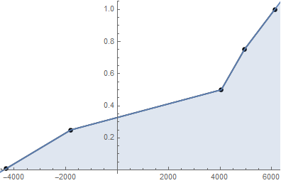
I'll take your data as five points of a CDF assigning kind of arbitrary probability values to the maximum loss and maximum profit values

data = {{-4305, 0.01}, {-1801, 0.25}, {4044, 0.5}, {4938, 0.75}, {6120, 1.00}}

and interpolate this data.

if = Interpolation[data, InterpolationOrder -> 1];

listPlot = ListPlot[data, Joined -> True, Mesh -> All, PlotStyle -> Black];
Show[listPlot, Plot[if[x], {x, -5000, 7000}, Filling -> Axis, PlotRange -> All]]
Out1

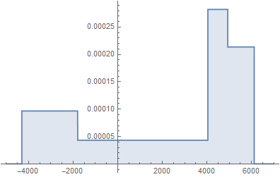
Using the interpolated data (if) to define a ProbabilityDistribution

pD = ProbabilityDistribution[{"CDF", if[x]}, {x, -4305, 6120}, Method -> "Normalize"];

Plot[PDF[pD], x], {x, -5000, 7000}, Filling -> Axis, PlotRange -> All]
Out2

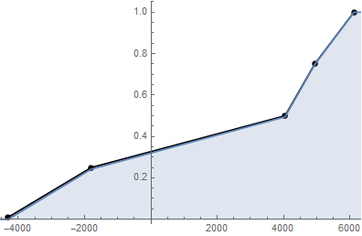
Show[{listPlot, Plot[CDF[pD], x], {x, -5000, 7000}, Filling -> Axis, PlotRange -> All]}]
Out3

One can use this ProbabilityDistribution (pD) to derive some additional statistics. For example

Through[{Mean, StandardDeviation, Quantile[#, {1/100, 1/4, 1/2, 3/4, 99/100}] &}[pD]]] // N

$\ ${2073.39, 3461.64, {-4201.71, -1625.65, 4061.88, 4949.82, 6073.19}}

Or create some pseudorandom variats from pD

rv = RandomVariate[pD, 100000];

and feed FindDistribution with them

{dist1, dist2, dist3} = FindDistribution[rv, 3]

Show[{listPlot, Plot[{CDF[dist1, x], CDF[dist2, x], CDF[dist3, x]}, {x, -8000, 8000}]}]
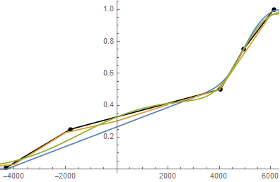
Out4

Plot[{PDF[dist1, x], PDF[dist2, x], PDF[dist3, x]}, {x, -8000, 8000}]
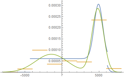
Out5

Through[{Mean, Median, StandardDeviation, Quantile[#, {1/100, 1/4, 1/2, 3/4, 99/100}]&}[dist1]]

$\ ${2355.22, 3724.49, 3104.68, {-4141.88, -231.04, 3724.49, 4937.08, 6093.1}}

Through[{Mean, Median, StandardDeviation, Quantile[#, {1/100, 1/4, 1/2, 3/4, 99/100}]&}[dist2]]

$\ ${2145.7, 4014.08, 3556.66, {-5328.89, -1409.09, 4014.08, 5077.46, 7396.}}

Through[{Mean, Median, StandardDeviation, Quantile[#, {1/100, 1/4, 1/2, 3/4, 99/100}]&}[dist3]]

$\ ${2102.4, 3907.54, 3468.62, {-5719.51, -1039.81, 3907.54, 4950.12, 6491.02}}


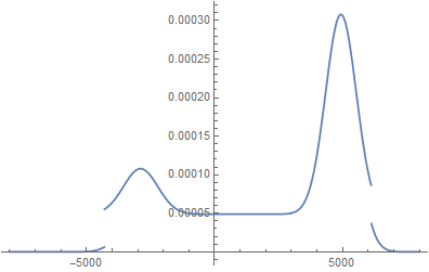
From another run of RandomVariate I got these PDFs: Out6
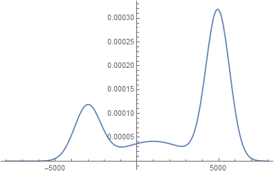
Out7

$\endgroup$
6
  • $\begingroup$ For the linear interpolation, I believe that the CDF should be data = {{-4305, 0}, {-1801, 0.25}, {4044, 0.5}, {4938, 0.75}, {6120, 1}}; cdf[p_] = Piecewise[{{1, p >= 6120}, {Interpolation[data, InterpolationOrder -> 1][p], -4305 < p < 6120}}]; $\endgroup$
    – Bob Hanlon
    Commented Nov 7, 2015 at 2:52
  • $\begingroup$ @BobHanlon In my opinion you are erring to the wrong side. I wouldn't assume that the probability of getting a loss equal or bigger than "Maximum loss" is 0. I think from the given data one can only conclude that the biggest loss within the backtest was -4305 and that it was reached for less than 25 % of the trades. I'm also convinced that one should always make sure that this tail is fat enough. If this is a strategy with unlimited loss that mean the probability of having a bigger loss is higher than 0 % and if it is a strategy with limited risk it means ... $\endgroup$
    – Karsten7
    Commented Nov 7, 2015 at 5:15
  • $\begingroup$ ... that the maximum loss probably occurs for a bigger percentage of trades. Your cdf is the correct way of creating a CDF directly from the data using Interpolation and it's an important point that my if should not be misinterpreted as a CDF, as its extrapolation will be incorrect. However, the PDF will be taken to be zero for values smaller than -4305 or bigger than 6120 by specifying {x, -4305, 6120} within pD = ProbabilityDistribution[{"CDF", if[x]}, {x, -4305, 6120}, Method -> "Normalize"];. $\endgroup$
    – Karsten7
    Commented Nov 7, 2015 at 5:30
  • $\begingroup$ @Karsten7. Congratulations! Amazing answer !!! $\endgroup$
    – Rod
    Commented Nov 8, 2015 at 19:56
  • $\begingroup$ @Karsten7., you can go link below to see what I have done based on your code. I would like to do a MonteCarlo analysis over hundreds/thousands of equity curves, but the memory limit in the free version of WolframCloud is the limiting factor right now. Here it is: wolframcloud.wolframcloud.com/objects/… $\endgroup$
    – pyrex
    Commented Nov 9, 2015 at 18:08

Your Answer

By clicking “Post Your Answer”, you agree to our terms of service and acknowledge you have read our privacy policy.

Not the answer you're looking for? Browse other questions tagged or ask your own question.