17
$\begingroup$

Short version: how to estimate the parameters of a mixture of multivariate normal distributions (i.e.: Gaussian mixture model)?


Long version.

I am trying to estimate the parameters of a mixture of multivariate Gaussian distribution.

I know how to do it for a single multivariate normal distribution:

dist = MultinormalDistribution[{0, 0}, {{1, 0}, {0, 1}}];
dataSet = RandomVariate[dist, 300];
estDist = EstimatedDistribution[dataSet, MultinormalDistribution[{m1, m2}, {s11, s12}, {s12, s22]}}]]

Plot[{PDF[dist, {x, 0}], PDF[estDist, {x, 0}]}, {x, -4, 4}, Filling -> Axis]
SmoothDensityHistogram[dataSet]
Plot3D[PDF[estDist, {x, y}], {x, -2, 2}, {y, -2, 2}]
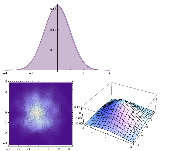
Similarity of PDF at y=0, density of dataset and estimated density.

All fine and dandy. However, the same approach does not work for me with mixture distributions. In particular, I am interested in mixtures of Gaussian distribution (Gaussian Mixture Model).

I generate a sample dataset:

targetDist = MixtureDistribution[{1/3, 2/3}, {MultinormalDistribution[{0, 0}, {{1, 0}, {0, 1}}], MultinormalDistribution[{3, 3}, {{1, 0}, {0, 1}}]}];
dataSet = RandomVariate[targetDist, 500];
ListPlot[dataSet]
SmoothHistogram3D[dataSet]
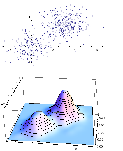
Mixture of Gaussians

I try to find the estimated distribution with:

estimatedDist = EstimatedDistribution[dataSet,
    MixtureDistribution[{w1, w2}, {
        MultinormalDistribution[{m11, m12}, {{s111, s112}, {s112, s122}}],
        MultinormalDistribution[{m21, m22}, {{s211, s212}, {s212, s222}}]
    }]]

But the evaluation always fails with:

NMaximize::cvdiv: Failed to converge to a solution. The function may be unbounded. >>

For some reason, it works if, instead of using MultinormalDistribution I use BinormalDistribution with $\rho$=0.

I know how to estimate these parameters using the Expectation Maximization algorithm, but I was wondering if there is a Mathematica-friendly way to do it.


Edit.

Giving initial estimates of the parameters does not really improve much. Even when giving the exact parameters like this:

estimatedDist = EstimatedDistribution[dataSet, 
    MixtureDistribution[
        {w1, w2},
        {MultinormalDistribution[{m11, m12}, {{s111, s112}, {s121, s122}}],
         MultinormalDistribution[{m21, m22}, {{s211, s212}, {s221, s222}}]}],
        {{w1, 1/3}, {w2, 2/3}, {m11, 0}, {m12, 0}, {s111, 1}, {s112, 0}, {s121, 0}, {s122, 1}, {m21, 3}, {m22, 3}, {s211, 1}, {s212, 0}, {s221, 0}, {s222, 1}}]

EstimatedDistribution seems to take much more time than what it would be reasonable (and, since the estimates are exact, "reasonable" means 0.1 sec).

After about 15 minutes of processing on a 3.3GHz Xeon, I got this error:

FindMaximum::eit: The algorithm does not converge to the tolerance of
4.806217383937354`*^-6 in 500 iterations. The best estimated solution,
with feasibility residual, KKT residual, or complementary residual of
{2.1536*10^-12,0.00200273,5.6281*10^-13}, is returned. >>

Then a popup message:

INTERNAL SELF-TEST ERROR: MLParseStream|c|297
Click here to find out if this problem is known, and to help improve
Mathematica by reporting it to Wolfram Research.
$\endgroup$
2
  • $\begingroup$ You are aware that you can supply EstimatedDistribution[] with initial estimates of parameters? $\endgroup$ Commented Nov 22, 2012 at 14:19
  • $\begingroup$ @J.M. Please see my edit. Using the exact parameters as estimation seems just to avoid divergence, but EstimatedDistribution still fails to return a meaningful result. $\endgroup$ Commented Nov 22, 2012 at 15:15

3 Answers 3

14
$\begingroup$

You need to make sure that the constraints on the parameters are satisfied. In this case, these are

1) The mixture weights sum to one. 2) The covariance matrices of the two bivariate normals need to be positive definite.

The first constraint can be guaranteed by specifying the weights as follows:

w1 = Exp[w]/(1 + Exp[w]);

where w is unconstrained.

The second constraint can be enforced by using the Cholesky Decomposition of the covariance matrices as below.

c1 = {{c111, 0}, {c112, c122}};

where c1 is a lower triangular matrix of unrestricted elements. The resulting covariance matrix is given by s1 below.

s1 = c1.Transpose[c1]

Out[9]= {{c111^2, c111 c112}, {c111 c112, c112^2 + c122^2}}

Similarly, we have for the other covariance,

s2 = c2.Transpose[c2];

Let the two mean vectors be

m1 = {m11, m12};

m2 = {m21, m22};

The mixture pdf can be written as

In[15]:= mixPDF = MixtureDistribution[{w1, 1 - w1}, 
  {MultinormalDistribution[m1, s1], 
   MultinormalDistribution[m2, s2]
   }
  ]

Out[15]= MixtureDistribution[{E^w/(1 + E^w), 
  1 - E^w/(1 + E^w)}, {MultinormalDistribution[{m11, 
    m12}, {{c111^2, c111 c112}, {c111 c112, c112^2 + c122^2}}], 
  MultinormalDistribution[{m21, 
    m22}, {{c211^2, c211 c212}, {c211 c212, c212^2 + c222^2}}]}]

Then one may get what you are looking for, depending upon starting values.. The first try here does not give the correct answer.

In[16]:= est1 = EstimatedDistribution[dataSet, mixPDF]

Out[16]= MixtureDistribution[{0.0172133, 
  0.982787}, {MultinormalDistribution[{1.37871, 
    0.821044}, {{4.88591, 1.35155}, {1.35155, 0.373881}}], 
  MultinormalDistribution[{1.91595, 
    1.88312}, {{3.0206, 2.01692}, {2.01692, 3.08025}}]}]

Specifying starting values helps.

In[17]:= est2 = 
 EstimatedDistribution[dataSet, 
  mixPDF, {{m11, - 0.5}, {m12, 0.8}, {m21, 1.5}, {m22, 2.0}, {c111, 
    1.5}, {c112, 0.0}, {c122, 1.0}, {c211, 1.5}, {c212, 0.0}, {c222, 
    1.0}, {w, 0.2}}]

Out[17]= MixtureDistribution[{0.39772, 
  0.60228}, {MultinormalDistribution[{0.110727, 
    0.110757}, {{1.05393, 0.060291}, {0.060291, 1.07923}}], 
  MultinormalDistribution[{3.0927, 
    3.02315}, {{0.84418, -0.148054}, {-0.148054, 0.982491}}]}]

An alternative approach can use FindDistributionParameters as follows

In[18]:= 
est3 = FindDistributionParameters[dataSet, 
  mixPDF, {{m11, 0.0}, {m12, 0.0}, {m21, 2.5}, {m22, 3.0}, {c111, 
    1.5}, {c112, 0.0}, {c122, 1.0}, {c211, 1.5}, {c212, 0.0}, {c222, 
    1.0}, {w, 0.5}}]

Out[18]= {m11 -> 0.110727, m12 -> 0.110757, m21 -> 3.0927, 
 m22 -> 3.02315, c111 -> 1.02661, c112 -> 0.0587281, c122 -> 1.0372, 
 c211 -> 0.918792, c212 -> -0.16114, c222 -> 0.978021, w -> -0.414975}

The original parameters can be obtained as

In[19]:= {w1, 1 - w1, m1, s1, m2, s2} /. est3

Out[19]= {0.39772, 0.60228, {0.110727, 
  0.110757}, {{1.05393, 0.060291}, {0.060291, 1.07923}}, {3.0927, 
  3.02315}, {{0.84418, -0.148054}, {-0.148054, 0.982491}}}
$\endgroup$
1
  • 3
    $\begingroup$ This is a great answer. I hadn't realized that EstimatedDistribution doesn't take sensible constraints on the parameters into account. So, I assume that we have to use similar tactics for other distributions, right? Like n>=0 for the binomial distribution and sigma >=0 for normal distribution. $\endgroup$ Commented Jul 3, 2013 at 21:03
3
$\begingroup$

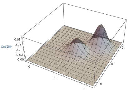
It's worth noting that since version 12, you can use LearnDistribution for this. It's not so easy to extract the distribution parameters from the result, but if you just need to fit a PDF to some data it's very easy to use and quite robust:

targetDist = MixtureDistribution[{1/3, 2/3},
 {
    MultinormalDistribution[{0, 0}, {{1, 0}, {0, 1}}], 
    MultinormalDistribution[{3, 3}, {{1, 0}, {0, 1}}]
  }
];
dataSet = RandomVariate[targetDist, 500];
dist = LearnDistribution[dataSet, Method -> "GaussianMixture"];
Plot3D[PDF[dist, {x, y}], {x, -6, 6}, {y, -6, 6}, PlotRange -> All, 
 PlotStyle -> Directive[Gray, Opacity[0.5]], PlotPoints -> 25]

enter image description here

Edit

With a little bit more effort, you can recover the fit parameters from the learned model as well:

ClearAll[fitGaussianMixture];
fitGaussianMixture[data_List, n_Integer, opts : OptionsPattern[LearnDistribution]] := Module[{
   fit = LearnDistribution[dataSet,
     Method -> {
        "GaussianMixture", "ComponentsNumber" -> n,
        "CovarianceType" -> "Full"
     },
     FeatureExtractor -> "Minimal",
     opts
   ],
   globalMean,
   means, covariances, weights
  },
  Condition[
    globalMean = fit[[1, "Model", "Processor", 2, "Mean"]];
    means = # + globalMean & /@ fit[[1, "Model", "Means"]];
    covariances = Transpose[#].# & /@ fit[[1, "Model", "CholeskyCovariances"]];
    weights = fit[[1, "Model", "MixingCoefficients"]];
    MixtureDistribution[
      weights,
      MapThread[
        MultinormalDistribution,
        {means, covariances}
      ]
    ]
    ,
    Head[fit] === LearnedDistribution
  ]
];

dist = fitGaussianMixture[dataSet, 2]

MixtureDistribution[{0.692171, 0.307829}, {MultinormalDistribution[{2.96774, 3.06928}, {{1.00801, -0.00695319}, {-0.00695319, 1.02726}}], MultinormalDistribution[{-0.0960511, -0.0773903}, {{1.07884, -0.0850454}, {-0.0850454, 0.902474}}]}]

$\endgroup$
2
$\begingroup$

You may have more success creating your own custom mixture distribution.

Oleksandr Pavlyk created a presentation about creating distributions in Mathematica for the Wolfram Technology Conference 2011 workshop:

'Create Your Own Distribution'.

You can download it here.

The downloads include the notebook,

'ExampleOfParametricDistribution.nb'

that seems to lay out all the pieces required to create a distribution that one can use like the distributions that come with Mathematica.

It takes some time and thought to set up all of the pieces, but once done your custom distribution can work like a charm.

$\endgroup$
4
  • $\begingroup$ I think that defining a new distribution would be much more difficult that implementing the EM algorithm, which is relatively simple. $\endgroup$ Commented Nov 23, 2012 at 20:13
  • $\begingroup$ I cant seem to find the .nb file? $\endgroup$ Commented Dec 19, 2014 at 1:04
  • 1
    $\begingroup$ @ChenStatsYu -- Send me an email and I can send you the notebook. You can find my address in my profile. $\endgroup$
    – Jagra
    Commented Dec 19, 2014 at 14:04
  • $\begingroup$ @Jagra Sorry about the confusion. I finally got the notebook. I will give it a go. I am having some trouble optimizing a likelihood from a mixture distribution. I wonder define an implicit PDF will have a better way to find mle. $\endgroup$ Commented Dec 19, 2014 at 14:17

Your Answer

By clicking “Post Your Answer”, you agree to our terms of service and acknowledge you have read our privacy policy.

Not the answer you're looking for? Browse other questions tagged or ask your own question.