4
$\begingroup$

I have some data (1593 values). I first binned it using the Knuth rule and fitted a function that is a linear combination of two sinh-arcsinh functions. I then rounded the resulting parameters to perform a FindDistributionParameters search of parameters using "MaximumLikelihood" as a ParameterEstimator. The problem is that after a lengthy computation I get an error message:

FindMaximum::eit: "The algorithm does not converge to the tolerance of 4.806217383937354`*^-6 in 100 iterations. The best estimated solution, with feasibility residual, KKT residual, or complementary residual of {8.33678,100.,4.16864}, is returned.

Unfortunately, there's no such thing like MaxIterations->Infinity in FindDistributionParameters.

The suitable code below; file.txt available here

import = Import["file.txt", "Table"];
data = Flatten[import];
data = Log[10, data];
data = Delete[data, Position[data, RankedMin[data, 1]][[1, 1]]];
data = Delete[data, Position[data, RankedMax[data, 1]][[1, 1]]];

sas[μ_, σ_, skew_, kurt_] := 
ProbabilityDistribution[((1 + ((z - μ)/σ)^2)^(-(1/2))
kurt Cosh[
kurt ArcSinh[(z - μ)/σ] - 
skew] Exp[-(1/2) Sinh[
kurt ArcSinh[(z - μ)/σ] - skew]^2])/(
Sqrt[2 π] σ), {z, -Infinity, Infinity}]

dist = MixtureDistribution[{p, 
1 - p}, {sas[μ1, σ1, skew1, kurt1], 
sas[μ2, σ2, skew2, kurt2]}]

param = FindDistributionParameters[data, 
dist, {{μ1, -0.2}, {σ1, 0.7}, {skew1, 0.3}, {kurt1, 
1.}, {μ2, 1.5}, {σ2, 0.5}, {skew2, 0.}, {kurt2, 
1.}, {p, 0.25}}, 
ParameterEstimator -> {"MaximumLikelihood", 
Method -> "NMaximize"}]

I'm not sure whether the error may be ignored, or it implies that there is room for a significant improvement of the obtained result. If the error may be dealt with, what's the solution?

$\endgroup$
4
  • 1
    $\begingroup$ ...because your PDF isn't numerical anywhere... try this PDF[sas[0.1, 1, 0.3, 0.4], 10] and you'll see there's a symbolic \[Sigma]1 lurking there. If we change the ... Sqrt[2 \[Pi]] \[Sigma]1) ... to Sqrt[2 \[Pi]] \[Sigma]) we can now get values out and do stuff like Plot[PDF[sas[0.1, 1, 0.3, 0.4], x], {z, -10, 10}] . I can't help with the rest of the problem if I don't have some values for data. $\endgroup$
    – Histograms
    Commented May 24, 2015 at 16:54
  • $\begingroup$ A very relevant answer here. All answers below that simply use p and 1-p are doing it wrong. $\endgroup$ Commented May 24, 2015 at 22:40
  • $\begingroup$ @SjoerdC.deVries are you talking about answers here or in that thread? I enforced 0 <= p <= 1 in the assumptions and since we're restricting it to a two-mixture p and 1-p are surely adequate weights. We can't make any assumptions on the dependency or use the Bayes' rule because we don't have the original classes the data came from. $\endgroup$
    – Histograms
    Commented May 25, 2015 at 0:03
  • $\begingroup$ @Histogram I have to retract that statement. I was in a bit of hurry when I wrote that and had only glanced over the answers seeing a mixture distribution with p and 1-p twice. I knew that FindDistributionParameters was not going to work in that way and that the method described in the link was the way to go. I see now that both of you do something different. It is still relevant for the approach used by the OP though. The nice thing of the trick is that there is no need for hard conditions on p which may make maximizing a bit easier. It might also work in your approach. $\endgroup$ Commented May 25, 2015 at 6:59

2 Answers 2

4
$\begingroup$

I rewrote quite a few things... manually specifying the mixture, and setting very low iteration and precision goals because it hangs for what seems like an eternity. Importantly I also specified assumptions on the distribution:

sas[μ_, σ_, skew_, kurt_, 
  z_] := ((1 + ((z - μ)/σ)^2)^(-(1/2)) kurt Cosh[
     kurt ArcSinh[(z - μ)/σ] - 
      skew] Exp[-(1/2) Sinh[
        kurt ArcSinh[(z - μ)/σ] - skew]^2])/(Sqrt[
     2 π] σ)

(*dist=MixtureDistribution[{p,1-p},{sas[μ1,σ1,skew1,kurt1],\
sas[μ2,σ2,skew2,kurt2]}]*)
dist[p_, μ1_, μ2_, σ1_, σ2_, skew1_, skew2_, 
  kurt1_, kurt2_] := 
 ProbabilityDistribution[
  p*sas[μ1, σ1, skew1, kurt1, z] + (1 - p)*
    sas[μ2, σ2, skew2, kurt2, z], {z, -Infinity, Infinity},
   Assumptions -> {σ1 > 0, σ2 > 0, skew1 >= 0, 
    skew2 >= 0, kurt1 >= 0, kurt2 >= 0, 0 <= p <= 1}]


param = FindDistributionParameters[data, 
  dist[p, μ1, μ2, σ1, σ2, skew1, skew2, kurt1, 
   kurt2], {{μ1, -0.2}, {σ1, 0.7}, {skew1, 0.3}, {kurt1, 
    1.}, {μ2, 1.5}, {σ2, 0.5}, {skew2, 0.}, {kurt2, 
    1.}, {p, 0.25}}, 
  ParameterEstimator -> {"MaximumLikelihood", 
    Method -> {"NMaximize", PrecisionGoal -> 1, MaxIterations -> 5}}]
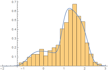
Show[Histogram[data, Automatic, "PDF"], 
 Plot[PDF[dist[p, μ1, μ2, σ1, σ2, skew1, skew2, 
     kurt1, kurt2] /. param, 
   z], {z, -2, 3}], PlotRange -> All]

enter image description here

$\endgroup$
3
  • 1
    $\begingroup$ I left it running while I was having dinner... these are the best parameters I got. DistributionFitTest will take forever, so if anyone wants to hack that be my guest: {kurt1 -> 2.76438, kurt2 -> 2.88617, p -> 0.643719, skew1 -> 0.513876, skew2 -> 1.39682, \[Mu]1 -> 1.23439, \[Mu]2 -> -0.997663, \[Sigma]1 -> 1.54076, \[Sigma]2 -> 2.92329} $\endgroup$
    – Histograms
    Commented May 24, 2015 at 20:00
  • $\begingroup$ Why did you use ProbabilityDistribution instead of my initial MixtureDistribution? Is computationally more efficient? $\endgroup$
    – corey979
    Commented May 24, 2015 at 20:18
  • 1
    $\begingroup$ god knows, I just wanted to be sure it wasn't some weird problem with MixtureDistribution, you can probably change that with no issues. $\endgroup$
    – Histograms
    Commented May 24, 2015 at 20:31
2
$\begingroup$

If you only need an estimate of the density function as opposed to estimates and standard errors for the coefficients of a specified model structure, then obtaining a kernel density estimate might be all you need.

(* Define distribution *)
sas[μ_, σ_, skew_, kurt_] := ProbabilityDistribution[
  ((1 + ((z - μ)/σ)^2)^(-(1/2)) kurt Cosh[
      kurt ArcSinh[(z - μ)/σ] - skew]
      Exp[-(1/2) Sinh[
         kurt ArcSinh[(z - μ)/σ] - skew]^2])/(Sqrt[
      2 π] σ),
  {z, -Infinity, Infinity}]

(* Mixture distibution *)
dist = MixtureDistribution[{p, 1 - p}, {sas[μ1, σ1, skew1, kurt1], 
    sas[μ2, σ2, skew2, kurt2]}];

(* Generate some data *)
data = RandomVariate[
   dist /. {p -> 0.25, μ1 -> -0.2, σ1 -> 0.7, skew1 -> 0.3,
      kurt1 -> 1, μ2 -> 1.5, σ2 -> 0.5, skew2 -> 0, kurt2 -> 1}, 1593];

(* Histogram *)
p1 = Histogram[data, Automatic, "PDF"];

(* Nonparametric density estimate *)
d = SmoothKernelDistribution[data];
p2 = Plot[PDF[d, x], {x, -2, 3.2}];

(* Show both figures *)
Show[{p1, p2}]

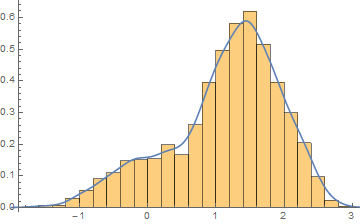
Kernel density estimate

This is not an answer to the specific question you have but does provide an alternative which avoids the error you see (not to mention avoiding the lengthy computation time).

$\endgroup$

Your Answer

By clicking “Post Your Answer”, you agree to our terms of service and acknowledge you have read our privacy policy.

Not the answer you're looking for? Browse other questions tagged or ask your own question.